Lanczos (pronounced Lanchos) resampling is a sophisticated technique for interpolating digital signals, offering superior image quality compared to simpler methods like nearest neighbor and bilinear interpolation. By effectively preserving detail and minimizing aliasing artifacts, Lanczos resampling is widely used in image and signal processing applications.
While Lanczos excels in image quality, it comes at the cost of increased computational complexity. Additionally, the potential for "ringing" artifacts, particularly around sharp edges, can be a drawback. Despite these challenges, Lanczos remains a preferred choice for tasks such as image scaling and rotation due to its overall performance benefits.
This document provides a comprehensive overview of Lanczos resampling, including its theoretical underpinnings, implementation details, and practical applications. It serves as a valuable resource for developers and researchers seeking to understand and utilize this powerful technique. The subsequent sections delve into crucial aspects of Lanczos resampling, such as the Lanczos kernel, interpolation and resampling processes, flux preservation, upsampling, downsampling, sample positioning, output range, multidimensional interpolation, and separability. A practical example with accompanying source code is included.
The Lanczos kernel, defined for a given support size, is a function used in Lanczos resampling. The kernel is defined as:
L(x) = sinc(x)*sinc(x/a) : -a < x < a
     = 0.0               : otherwise
Where:
The normalized sinc function is defined as:
sinc(x) = 1.0              : x = 0.0
        = sin(PI*x)/(PI*x) : otherwise

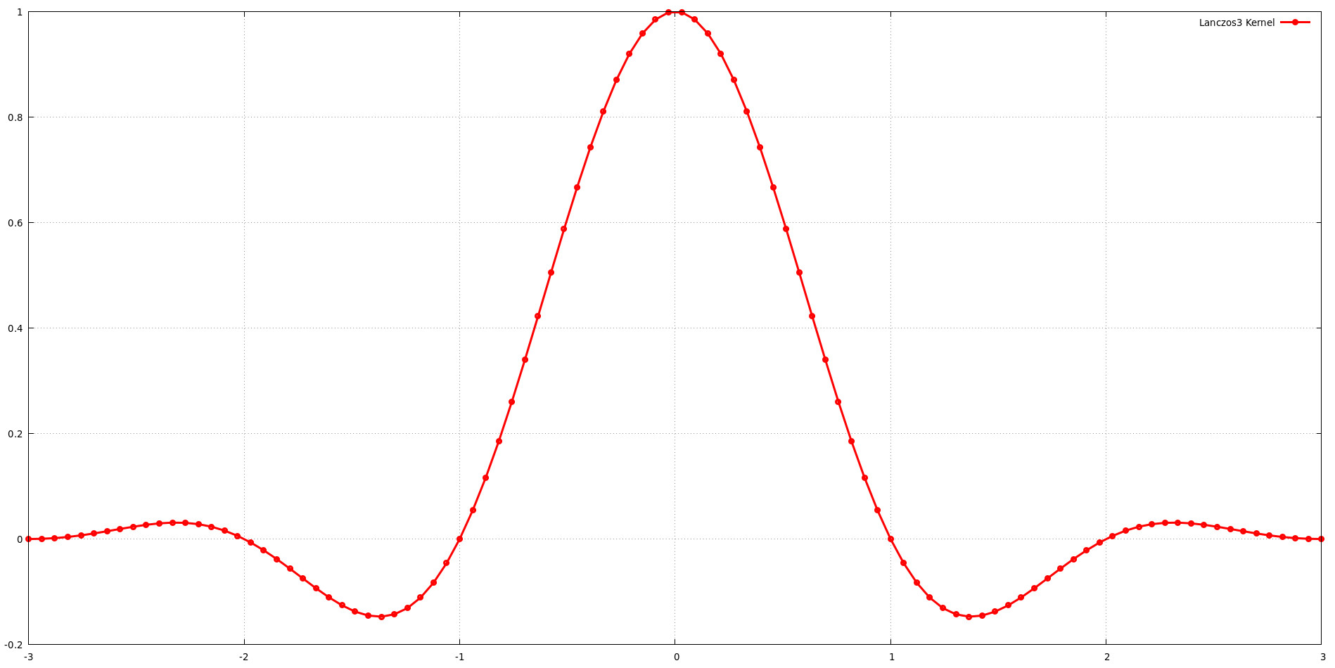
The graph illustrates the shape of the Lanczos kernel for a support size of a = 3. This means the kernel includes three lobes of the sinc function. While increasing the support size (a) generally provides more flexibility for shaping the frequency response, it also increases computational cost. A balance must be struck between image quality and computational efficiency when choosing the support size. Jim Blinn's finding that the Lanczos kernel with a = 3 offers an excellent balance of low-frequency preservation and high-frequency rejection supports this notion.
Note: The terms "kernel width," "support size," and "filter size" are often used interchangeably to describe the parameter a. However, in the context of Lanczos resampling, "support size" most accurately reflects the concept.
Lanczos interpolation is a technique used to resample a discrete signal to a new sampling rate. It achieves this by convolving the original signal with a Lanczos kernel.
The interpolated signal s2(x) can be calculated as follows:
s2(x) = (1/w(x))*
        SUM(i = -a + 1, i = a,
            s1(floor(x) + i)*
            L(i - x + floor(x)))
Where:
Preserving Flux:
The normalization factor w(x) is crucial for preserving the overall signal energy or mass during the interpolation process. It ensures that the sum of the interpolated values approximates the sum of the original samples. The filter weight is calculated as:
w(x) = SUM(i = -a + 1, i = a, L(i - x + floor(x)))
Upsampling:
When increasing the sampling rate, the Lanczos interpolation equation can be used directly without modifications.
Downsampling:
To avoid aliasing artifacts when decreasing the sampling rate, the filter scale must be adjusted to match the new sampling rate.
fs = n1/n2

s2(x) = (1/w(x))*
        SUM(i = -(fs*a) + 1, i = (fs*a),
            s1(floor(x) + i)*
            L((i - x + floor(x))/fs))
Where:
When resampling a signal from n1 samples to n2 samples the following sample positions are used. The index j is used to represent the samples from the sampled signal s2(x). The term (j + 0.5) is the center of a sample in s2(x). The step scales a point in s2(x) to a point in s1(x). The final -0.5 term in x is a phase shift that causes the Lanczos coefficient samples to be offset.
step = n1/n2
j    = [0..n2)
x    = (j + 0.5)*step - 0.5
When performing Lanczos interpolation, special care must be taken at the signal boundaries. Common edge handling techniques include:
Zero Padding:
s1(x) = s1[floor(x)] : x = [0, n1)
      = 0.0          : otherwise
Clamping:
s1(x) = s1[clamp(floor(x), 0, n1 - 1)]
Clamping is often preferred as it reduces edge artifacts caused by sharp discontinuities near the edges. However, the choice of edge handling method depends on the specific application and desired output.
The range of s2(x) may be greater than that of s1(x) due to the lobes of L(x). For example, an input signal s1(x) corresponding to pixel colors in the range of [0.0,1.0] need to be clamped to the same range to ensure that the output values do not overflow when converted back to unsigned bytes of [0,255].
The Lanczos kernel can be extended to multiple dimensions to perform interpolation on images or higher-dimensional data.
The two-dimensional Lanczos kernel is defined as:
L(x, y) = sinc(sqrt(x^2 + y^2))*sinc(sqrt(x^2 + y^2)/a)
The interpolated signal s2(x, y) can be calculated using the following formula:
s2(x, y) = (1/w(x, y))*
           SUM(i = -a + 1, i = a,
               SUM(j = -a + 1, j = a,
                   s1(floor(x) + j, floor(y) + i)*
                   L(j - x + floor(x), i - y + floor(y))))
Where w(x, y) is the normalization factor calculated using the two-dimensional Lanczos kernel.
Unlike some interpolation methods, the Lanczos kernel is non-separable, meaning it cannot be factored into the product of one-dimensional kernels. This property generally leads to higher computational costs compared to separable kernels. To improve performance, some implementations approximate the Lanczos kernel by performing separate passes for the horizontal and vertical dimensions.
Horizontal Interpolation:
Vertical Interpolation:
Mathematical Representation:
s2(x, y) = (1/w(x))*
           SUM(j = -a + 1, j = a,
               s1(floor(x) + j, y)*
               L(j - x + floor(x)))

s3(x, y) = (1/w(y))*
           SUM(i = -a + 1, i = a,
               s2(x, floor(y) + i)*
               L(i - y + floor(y)))
Note that the normalization factors w(x) and w(y) are calculated using the one-dimensional Lanczos kernel.
Key Points:
Similarly, recursively resampling a signal multiple times, as commonly done for generating texture mipmaps, can also degrade image quality due to the accumulation of errors from each resampling step.
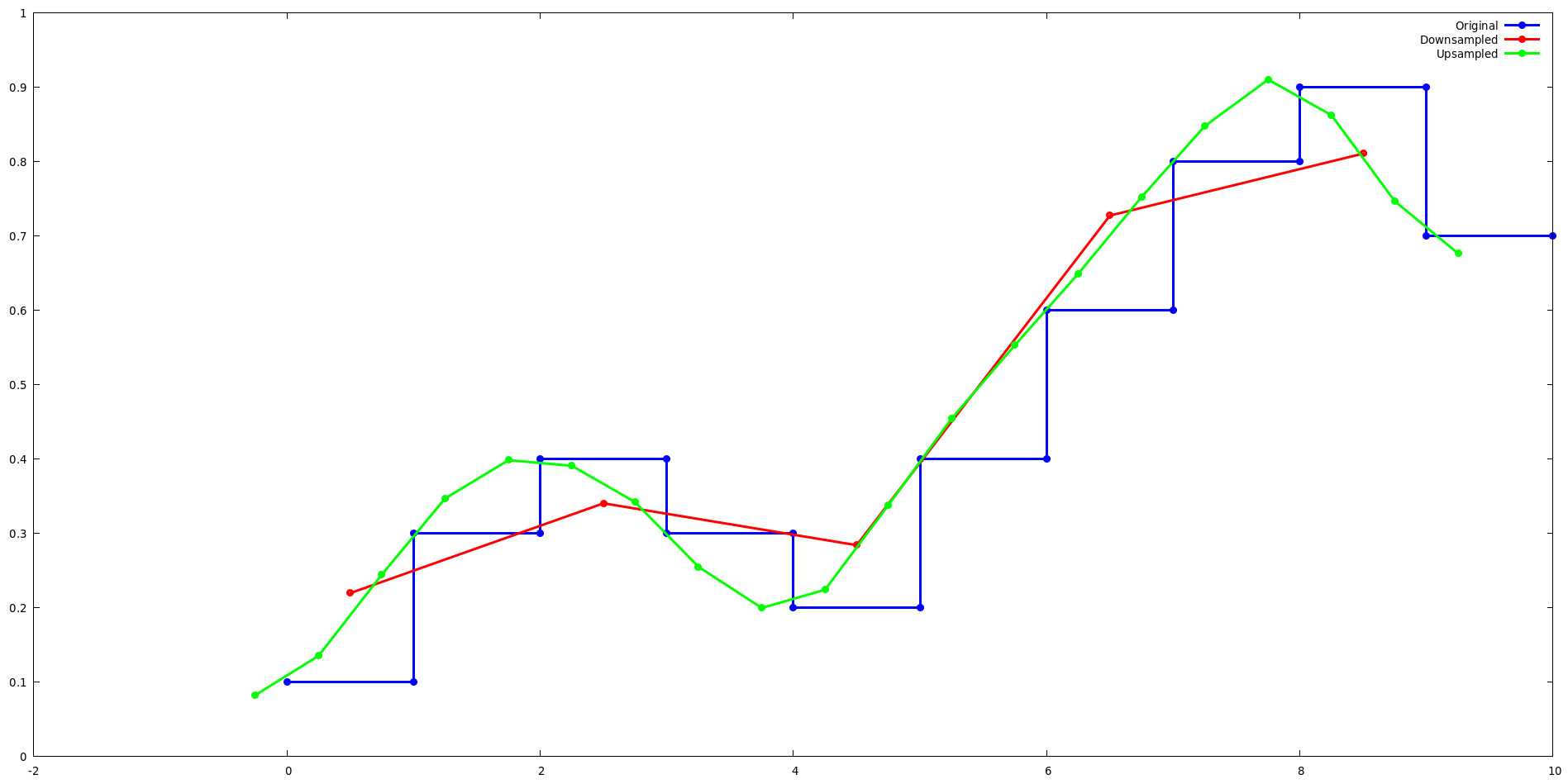
Run the lancos-test example and use gnuplot to see how Lanczos resampling affects a simple one-dimensional signal when upsampled and downsampled by a factor of 2.
make
./lanczos-test
gnuplot
> load "output.plot"

Upsampling:
When upsampling by a power-of-two, the Lanczos kernel cycles between 2^level sets of values. For example, consider the first 4 outputs of the lanzcos-test upsample example. Notice that the outputs for L(x) repeat for j={0,2} and j={1,3}.
upsample n1=10, n2=20
j=0, x=-0.250000
i=-2, L(-2.750000)=0.007356, S1(-3.000000)=0.100000
i=-1, L(-1.750000)=-0.067791, S1(-2.000000)=0.100000
i=0, L(-0.750000)=0.270190, S1(-1.000000)=0.100000
i=1, L(0.250000)=0.890067, S1(0.000000)=0.100000
i=2, L(1.250000)=-0.132871, S1(1.000000)=0.300000
i=3, L(2.250000)=0.030021, S1(2.000000)=0.400000
s2=0.082129, s2/w=0.082379, w=0.996972
j=1, x=0.250000
i=-2, L(-2.250000)=0.030021, S1(-2.000000)=0.100000
i=-1, L(-1.250000)=-0.132871, S1(-1.000000)=0.100000
i=0, L(-0.250000)=0.890067, S1(0.000000)=0.100000
i=1, L(0.750000)=0.270190, S1(1.000000)=0.300000
i=2, L(1.750000)=-0.067791, S1(2.000000)=0.400000
i=3, L(2.750000)=0.007356, S1(3.000000)=0.300000
s2=0.134869, s2/w=0.135279, w=0.996972
j=2, x=0.750000
i=-2, L(-2.750000)=0.007356, S1(-2.000000)=0.100000
i=-1, L(-1.750000)=-0.067791, S1(-1.000000)=0.100000
i=0, L(-0.750000)=0.270190, S1(0.000000)=0.100000
i=1, L(0.250000)=0.890067, S1(1.000000)=0.300000
i=2, L(1.250000)=-0.132871, S1(2.000000)=0.400000
i=3, L(2.250000)=0.030021, S1(3.000000)=0.300000
s2=0.243853, s2/w=0.244594, w=0.996972
j=3, x=1.250000
i=-2, L(-2.250000)=0.030021, S1(-1.000000)=0.100000
i=-1, L(-1.250000)=-0.132871, S1(0.000000)=0.100000
i=0, L(-0.250000)=0.890067, S1(1.000000)=0.300000
i=1, L(0.750000)=0.270190, S1(2.000000)=0.400000
i=2, L(1.750000)=-0.067791, S1(3.000000)=0.300000
i=3, L(2.750000)=0.007356, S1(4.000000)=0.200000
s2=0.345945, s2/w=0.346996, w=0.996972
Downsampling:
When downsampling by a power-of-two, the Lanczos kernel becomes independent of x since (x - floor(x)) becomes a constant which matches the phase shift. For example, consider the first 2 outputs of the lanzcos-test downsample example. Notice that the outputs of L(x) repeat for each j.
downsample n1=10, n2=5
j=0, x=0.500000
i=-5, L(-2.750000)=0.007356, S1(-5.000000)=0.100000
i=-4, L(-2.250000)=0.030021, S1(-4.000000)=0.100000
i=-3, L(-1.750000)=-0.067791, S1(-3.000000)=0.100000
i=-2, L(-1.250000)=-0.132871, S1(-2.000000)=0.100000
i=-1, L(-0.750000)=0.270190, S1(-1.000000)=0.100000
i=0, L(-0.250000)=0.890067, S1(0.000000)=0.100000
i=1, L(0.250000)=0.890067, S1(1.000000)=0.300000
i=2, L(0.750000)=0.270190, S1(2.000000)=0.400000
i=3, L(1.250000)=-0.132871, S1(3.000000)=0.300000
i=4, L(1.750000)=-0.067791, S1(4.000000)=0.200000
i=5, L(2.250000)=0.030021, S1(5.000000)=0.400000
i=6, L(2.750000)=0.007356, S1(6.000000)=0.600000
s2=0.437796, s2/w=0.219563, w=1.993943
j=1, x=2.500000
i=-5, L(-2.750000)=0.007356, S1(-3.000000)=0.100000
i=-4, L(-2.250000)=0.030021, S1(-2.000000)=0.100000
i=-3, L(-1.750000)=-0.067791, S1(-1.000000)=0.100000
i=-2, L(-1.250000)=-0.132871, S1(0.000000)=0.100000
i=-1, L(-0.750000)=0.270190, S1(1.000000)=0.300000
i=0, L(-0.250000)=0.890067, S1(2.000000)=0.400000
i=1, L(0.250000)=0.890067, S1(3.000000)=0.300000
i=2, L(0.750000)=0.270190, S1(4.000000)=0.200000
i=3, L(1.250000)=-0.132871, S1(5.000000)=0.400000
i=4, L(1.750000)=-0.067791, S1(6.000000)=0.600000
i=5, L(2.250000)=0.030021, S1(7.000000)=0.800000
i=6, L(2.750000)=0.007356, S1(8.000000)=0.900000
s2=0.678627, s2/w=0.340344, w=1.993943
As a further optimization, the Lanczos kernel may be precomputed for these cases to eliminate the expensive sinc function computation.
This README was created with the assistance of Google Gemini.
Additional references include:
This code was implemented by Jeff Boody under The MIT License.
Copyright (c) 2024 Jeff Boody

Permission is hereby granted, free of charge, to any person obtaining a
copy of this software and associated documentation files (the "Software"),
to deal in the Software without restriction, including without limitation
the rights to use, copy, modify, merge, publish, distribute, sublicense,
and/or sell copies of the Software, and to permit persons to whom the
Software is furnished to do so, subject to the following conditions:

The above copyright notice and this permission notice shall be included
in all copies or substantial portions of the Software.

THE SOFTWARE IS PROVIDED "AS IS", WITHOUT WARRANTY OF ANY KIND, EXPRESS OR
IMPLIED, INCLUDING BUT NOT LIMITED TO THE WARRANTIES OF MERCHANTABILITY,
FITNESS FOR A PARTICULAR PURPOSE AND NONINFRINGEMENT. IN NO EVENT SHALL THE
AUTHORS OR COPYRIGHT HOLDERS BE LIABLE FOR ANY CLAIM, DAMAGES OR OTHER
LIABILITY, WHETHER IN AN ACTION OF CONTRACT, TORT OR OTHERWISE, ARISING FROM,
OUT OF OR IN CONNECTION WITH THE SOFTWARE OR THE USE OR OTHER DEALINGS IN
THE SOFTWARE.