Create Waffle Chart Visualizations
Square pie charts (a.k.a. waffle charts) can be used to communicate parts of a whole for categorical quantities. To emulate the percentage view of a pie chart, a 10x10 grid should be used with each square representing 1% of the total. Modern uses of waffle charts do not necessarily adhere to this rule and can be created with a grid of any rectangular shape. Best practices suggest keeping the number of categories small, just as should be done when creating pie charts. Tools are provided to create waffle charts as well as stitch them together, and to use glyphs for making isotype pictograms.
It uses ggplot2 and returns a ggplot2 object.
The following functions are implemented:
waffle: Make waffle (square pie) charts
draw_key_pictogram: Legend builder for pictograms
fa_grep: Search Font Awesome glyph names for a pattern
fa_list: List all Font Awesome glyphs
fa5_brand: Font Awesome 5 Brand
fa5_solid: Font Awesome 5 Solid
geom_pictogram: Pictogram Geom
geom_waffle: Waffle (Square pie chart) Geom
install_fa_fonts: Install Font Awesome 5 Fonts
iron: Veritical, left-aligned layout for waffle plots
scale_label_pictogram: Used with geom_pictogram() to map Font
Awesome fonts to labels
theme_enhance_waffle: Waffle chart theme cruft remover that can be
used with any other theme
install.packages("waffle") # NOTE: CRAN version is 0.7.0
# or
remotes::install_github("hrbrmstr/waffle")
NOTE: To use the ‘remotes’ install options you will need to have the {remotes} package installed.
library(waffle)
library(magrittr)
library(hrbrthemes)
library(ggplot2)
library(dplyr)
library(waffle)

# current verison
packageVersion("waffle")
## [1] '1.0.2'data.frame(
parts = factor(rep(month.abb[1:3], 3), levels=month.abb[1:3]),
vals = c(10, 20, 30, 6, 14, 40, 30, 20, 10),
col = rep(c("navy", "black", "maroon"), 3),
fct = c(
rep("Thing 1", 3),
rep("Thing 2", 3),
rep("Thing 3", 3)
)
) -> xdf
xdf %>%
count(parts, wt = vals) %>%
ggplot(
aes(fill = parts, values = n)
) +
geom_waffle(
n_rows = 20,
size = 0.33,
colour = "white",
flip = TRUE
) +
scale_fill_manual(
name = NULL,
values = c("#a40000", "#c68958", "#ae6056"),
labels = c("Fruit", "Sammich", "Pizza")
) +
coord_equal() +
theme_ipsum_rc(grid="") +
theme_enhance_waffle()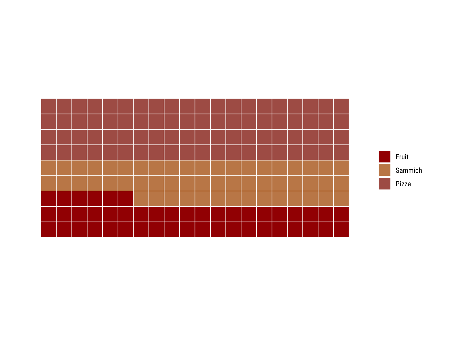
xdf %>%
  count(parts, wt = vals) %>%
  ggplot(
    aes(label = parts, values = n)
  ) +
  geom_pictogram(
    n_rows = 10,
    aes(colour = parts),
    flip = TRUE,
    make_proportional = TRUE
  ) +
  scale_color_manual(
    name = NULL,
    values = c("#a40000", "#c68958", "#ae6056"),
    labels = c("Fruit", "Sammich", "Pizza")
  ) +
  scale_label_pictogram(
    name = NULL,
    values = c("apple-alt", "bread-slice", "pizza-slice"),
    labels = c("Fruit", "Sammich", "Pizza")
  ) +
  coord_equal() +
  theme_ipsum_rc(grid="") +
  theme_enhance_waffle() +
  theme(
    legend.key.height = unit(2.25, "line"),
    legend.text = element_text(size = 10, hjust = 0, vjust = 0.75)
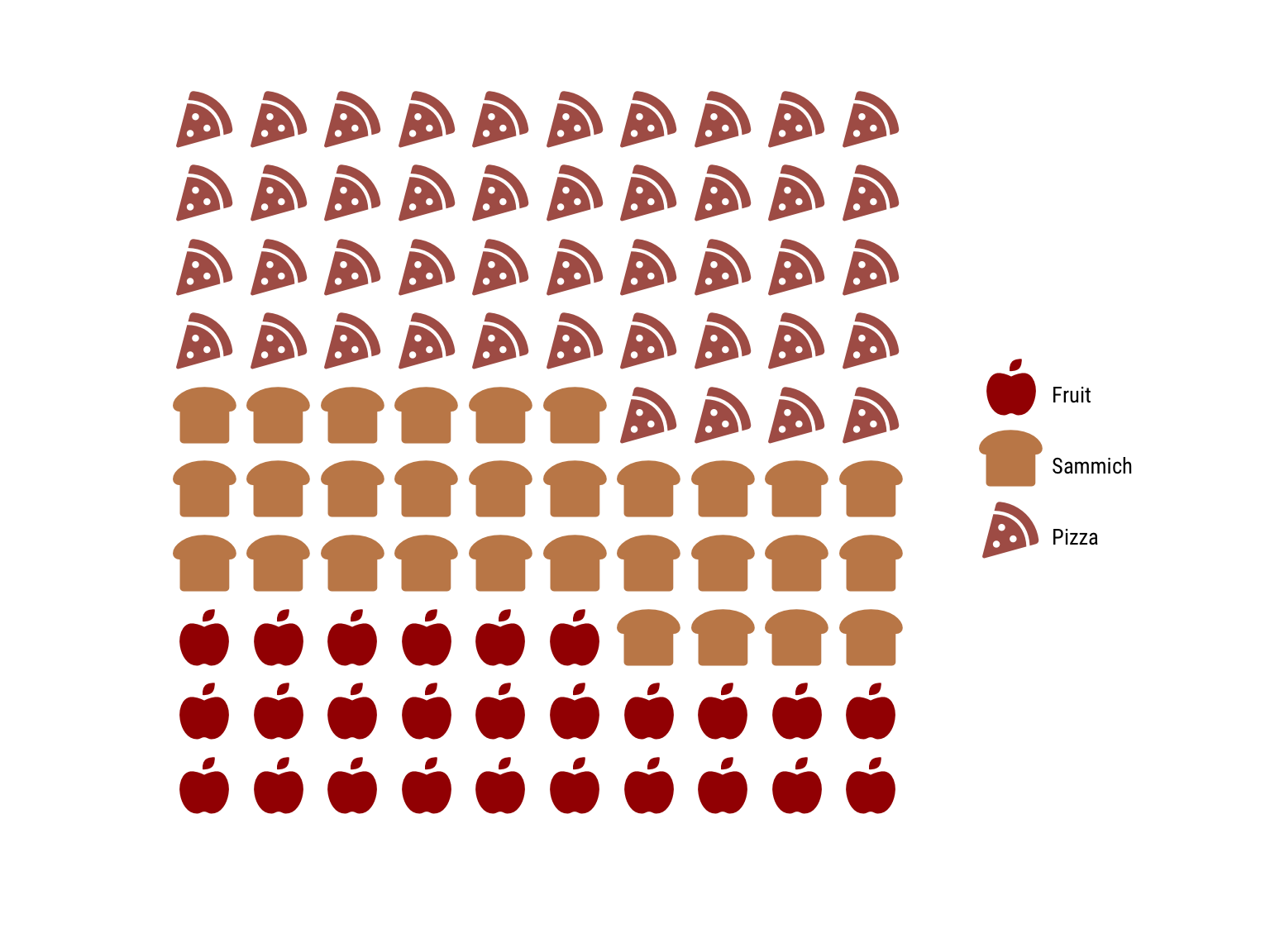
) 
xdf %>%
  count(parts, wt = vals) %>%
  ggplot(
    aes(label = parts, values = n)
  ) +
  geom_pictogram(
    n_rows = 20,
    size = 6,
    aes(colour = parts),
    flip = TRUE,
    family = "FontAwesome5Brands-Regular"
  ) +
  scale_color_manual(
    name = NULL,
    values = c("#073f9c", "black", "#f34323"),
    labels = c("BitBucket", "GitHub", "Other")
  ) +
  scale_label_pictogram(
    name = NULL,
    values = c("bitbucket", "github", "git-alt"),
    labels = c("BitBucket", "GitHub", "Other")
  ) +
  coord_equal() +
  theme_ipsum_rc(grid="") +
  theme_enhance_waffle() +
  theme(
    legend.text = element_text(hjust = 0, vjust = 1)
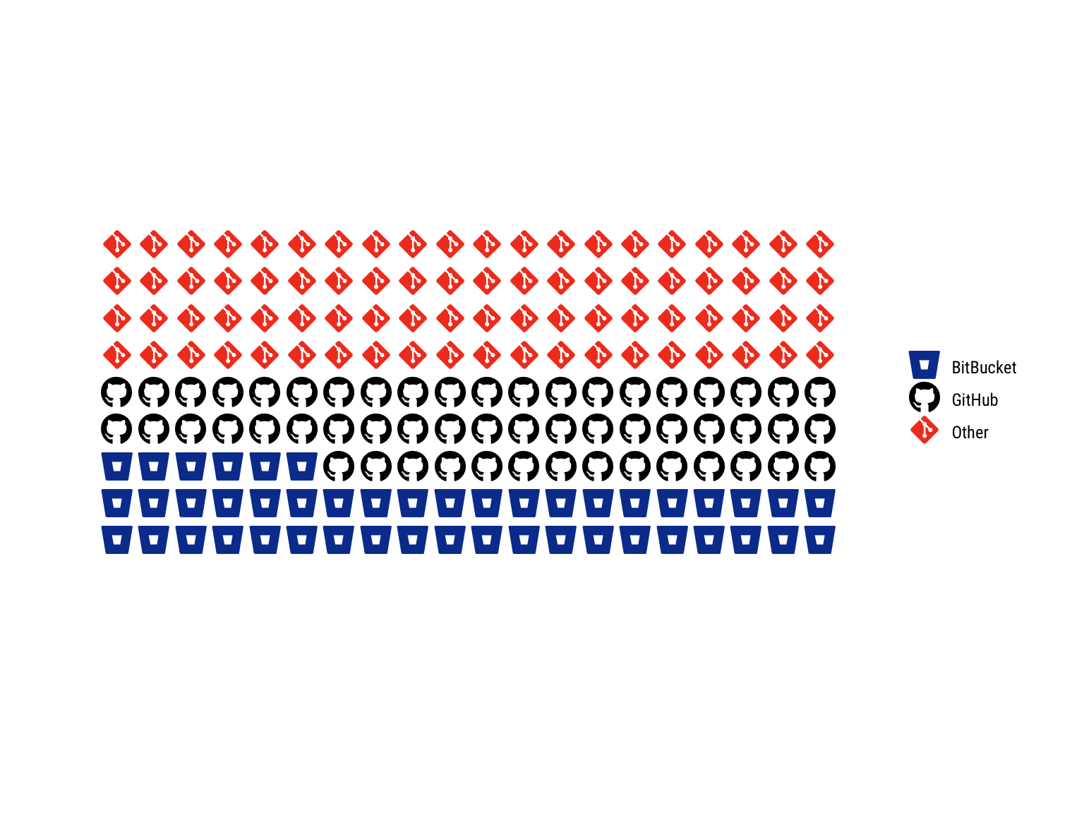
  )
library(hrbrthemes)
library(waffle)
library(tidyverse)

tibble(
  parts = factor(rep(month.abb[1:3], 3), levels=month.abb[1:3]),
  values = c(10, 20, 30, 6, 14, 40, 30, 20, 10),
  fct = c(rep("Thing 1", 3), rep("Thing 2", 3), rep("Thing 3", 3))
) -> xdf

ggplot(
  data = xdf,
  aes(fill=parts, values=values)
) +
  geom_waffle(
    color = "white",
    size = 1.125,
    n_rows = 6
  ) +
  facet_wrap(~fct, ncol=1) +
  scale_x_discrete(
    expand = c(0,0,0,0)
  ) +
  scale_y_discrete(
    expand = c(0,0,0,0)
  ) +
  ggthemes::scale_fill_tableau(name=NULL) +
  coord_equal() +
  labs(
    title = "Faceted Waffle Geoms"
  ) +
  theme_ipsum_rc(grid="") +
  theme_enhance_waffle()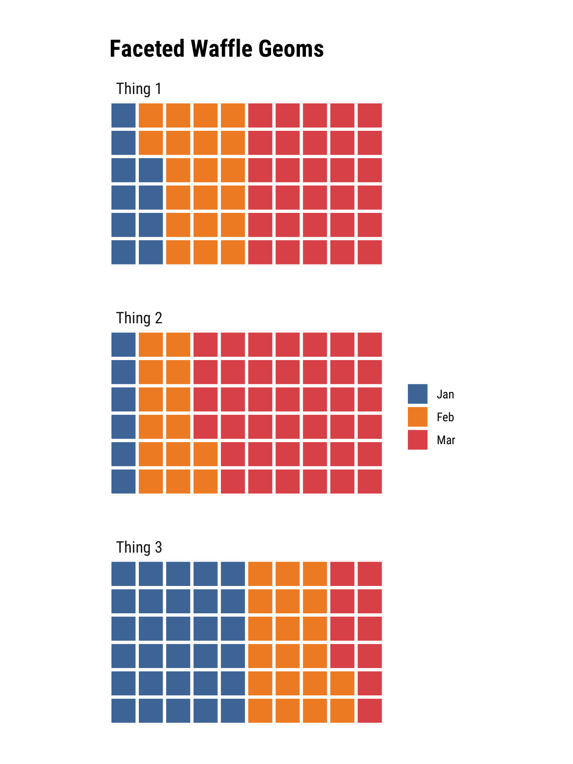
library(dplyr)
library(waffle)

storms %>%
  filter(year >= 2010) %>%
  count(year, status) -> storms_df

ggplot(
  data = storms_df,
  aes(fill = status, values = n)
) +
  geom_waffle(
    color = "white",
    size = .25,
    n_rows = 10,
    flip = TRUE
  ) +
  facet_wrap(
    ~year,
    nrow = 1,
    strip.position = "bottom"
  ) +
  scale_x_discrete() +
  scale_y_continuous(
    labels = function(x) x * 10, # make this multiplier the same as n_rows
    expand = c(0,0)
  ) +
  ggthemes::scale_fill_tableau(name=NULL) +
  coord_equal() +
  labs(
    x = "Year", y = "Count",
    title = "Faceted Waffle Bar Chart",
    subtitle = "{dplyr} storms data"
  ) +
  theme_minimal(
    base_family = "Roboto Condensed"
  ) +
  theme(
    panel.grid = element_blank(),
    axis.ticks.y = element_line()
  ) +
  guides(
    fill = guide_legend(reverse = TRUE)
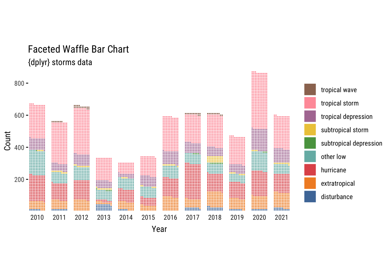
  )
parts <- c(80, 30, 20, 10)
waffle(parts, rows = 8)
parts <- data.frame(
  names = LETTERS[1:4],
  vals = c(80, 30, 20, 10)
)

waffle(parts, rows = 8)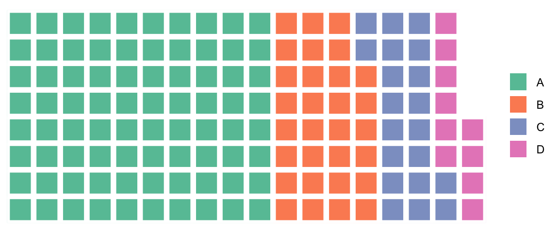
c(
  `Un-breachednUS Population` = (318 - 11 - 79),
  `Premera` = 11,
  `Anthem` = 79
) -> parts
waffle(
parts = parts,
rows = 8,
size = 1,
colors = c("#969696", "#1879bf", "#009bda"),
legend_pos = "bottom"
)Health records breaches as fraction of US Population

One square == 1m ppl
waffle(
  parts = parts / 10,
  rows = 3,
  colors = c("#969696", "#1879bf", "#009bda")
)
Health records breaches as fraction of US Population
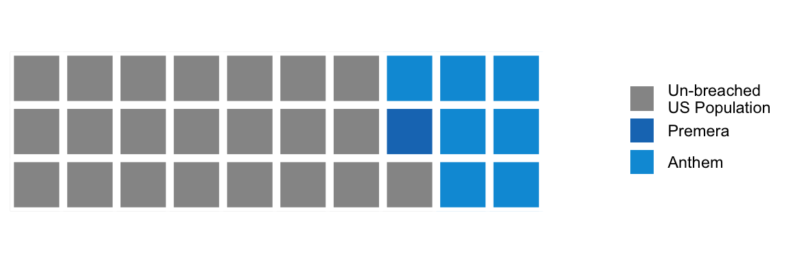
(One square == 10m ppl)
library(extrafont)

waffle(
  parts = parts / 10,
  rows = 3,
  colors = c("#969696", "#1879bf", "#009bda"),
  use_glyph = "medkit",
  size = 8
) +
  expand_limits(
    y = c(0, 4)
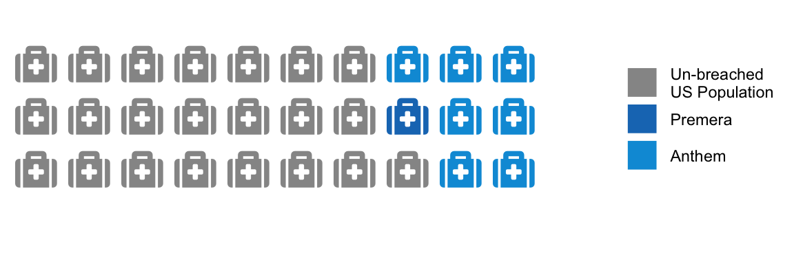
  )
Via: https://www.nytimes.com/2008/07/20/business/20debt.html
c(
  `Mortgagen($84,911)` = 84911,
  `Auto andntuition loansn($14,414)` = 14414,
  `Home equity loansn($10,062)` = 10062,
  `Credit Cardsn($8,565)` = 8565
) -> savings
waffle(
parts = savings / 392,
rows = 7,
size = 0.5,
legend_pos = "bottom",
colors = c("#c7d4b6", "#a3aabd", "#a0d0de", "#97b5cf")
)Average Household Savings Each Year

(1 square == $392)
Similar to https://eagereyes.org/techniques/square-pie-charts
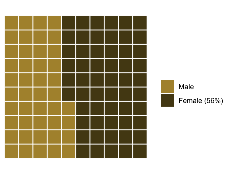
professional <- c(`Male` = 44, `Female (56%)` = 56)waffle(
parts = professional,
rows = 10,
size = 0.5,
colors = c("#af9139", "#544616")
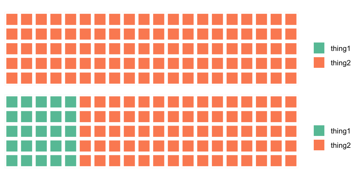
)With:
iron(
  waffle(
    parts = c(thing1 = 0, thing2 = 100),
    rows = 5
  ),
  waffle(
    parts = c(thing1 = 25, thing2 = 75),
    rows = 5
  )
)
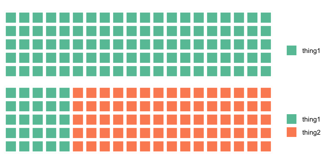
Without (you can disable this via keep parameter now):
iron(
  waffle(
    parts = c(thing1 = 0, thing2 = 100),
    rows = 5,
    keep = FALSE
  ),
  waffle(
    parts = c(thing1 = 25, thing2 = 75),
    rows = 5,
    keep = FALSE
  )
)
Professional Workforce Makeup
Iron example (left-align & padding for multiple plots)
pain.adult.1997 <- c(`YOY (406)` = 406, `Adult (24)` = 24)

waffle(
  parts = pain.adult.1997 / 2,
  rows = 7,
  size = 0.5,
  colors = c("#c7d4b6", "#a3aabd"),
  title = "Paine Run Brook Trout Abundance (1997)",
  xlab = "1 square = 2 fish", pad = 3
) -> A

pine.adult.1997 <- c(`YOY (221)` = 221, `Adult (143)` = 143)

waffle(
  parts = pine.adult.1997 / 2,
  rows = 7,
  size = 0.5,
  colors = c("#c7d4b6", "#a3aabd"),
  title = "Piney River Brook Trout Abundance (1997)",
  xlab = "1 square = 2 fish", pad = 8
) -> B

stan.adult.1997 <- c(`YOY (270)` = 270, `Adult (197)` = 197)

waffle(
  parts = stan.adult.1997 / 2,
  rows = 7,
  size = 0.5,
  colors = c("#c7d4b6", "#a3aabd"),
  title = "Staunton River Trout Abundance (1997)",
  xlab = "1 square = 2 fish"
) -> C

iron(A, B, C)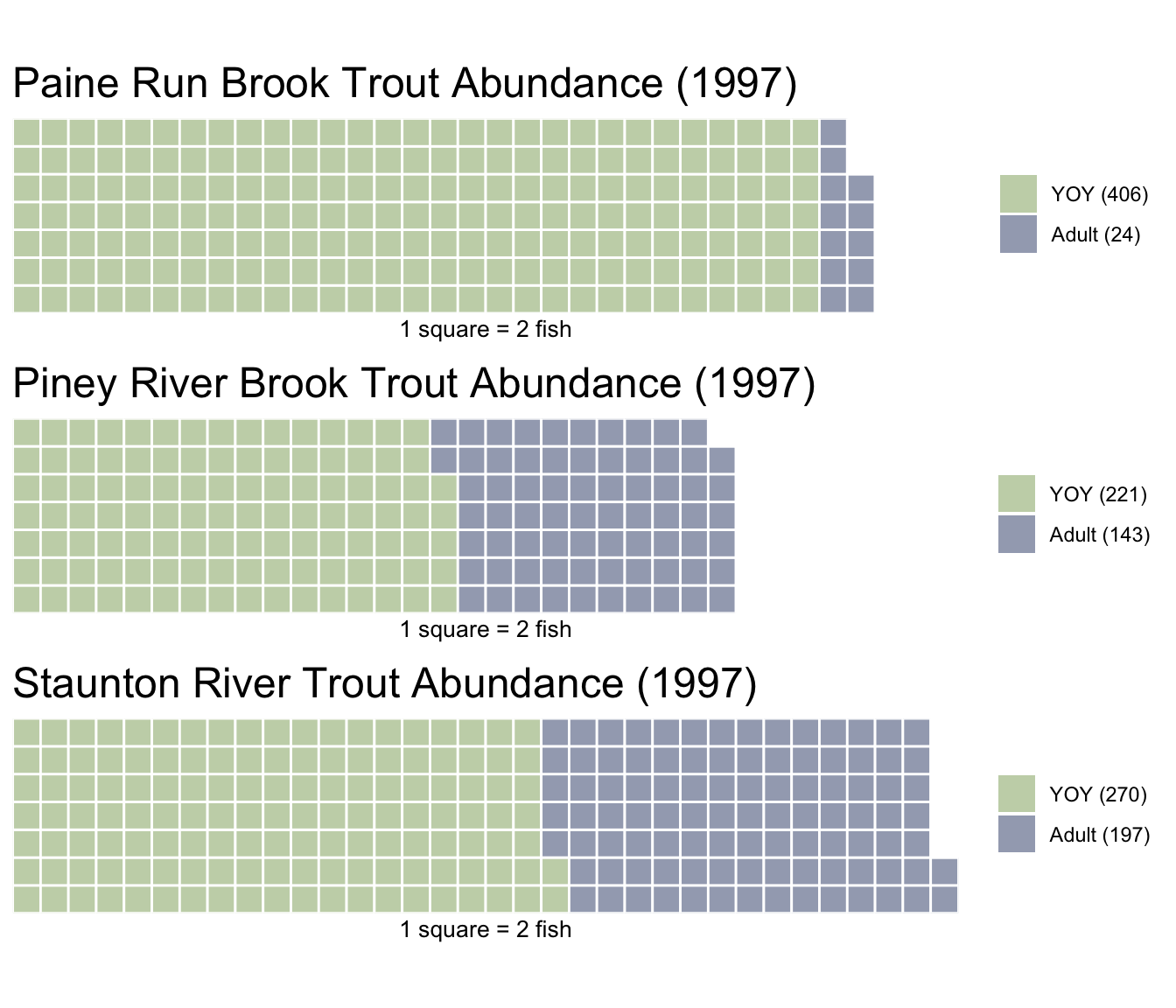
cloc::cloc_pkg_md()| Lang | # Files | (%) | LoC | (%) | Blank lines | (%) | # Lines | (%) |
|---|---|---|---|---|---|---|---|---|
| R | 14 | 0.44 | 624 | 0.35 | 218 | 0.36 | 439 | 0.38 |
| Rmd | 2 | 0.06 | 255 | 0.15 | 88 | 0.14 | 139 | 0.12 |
| SUM | 16 | 0.50 | 879 | 0.50 | 306 | 0.50 | 578 | 0.50 |
{cloc} ? metrics for waffle
Please note that this project is released with a Contributor Code of Conduct. By participating in this project you agree to abide by its terms.