smard power forecasting
1.0.0
This repository is for forecasting german power consumption.
Based and inspired from:
Data source: SMARD
Put all dowloaded files into:
/example/dataset # there is already used dataset included if you pull, but you could update
Check the forecast.Rmd file to see how you can run this code on a updated Version of SMARD-Data.
Used Libraries:
# Probably needed
# Load Packages
# library(fhswf)
# library(tsibbledata)
# library(broom)
# library(readr)
# library(datasets)
# library(timeDate)
# library(qlcal)
# library(corrplot)
# library(mgcv)
# library(MEFM)
# library(TTR)

packages <- c(
  "devtools",
  "ggplot2",
  "dplyr",
  "tsibble",
  "fable",
  "fabletools",
  "feasts",
  "distributional",
  "lubridate",
  "tidyr",
  "forecast",
  "zoo",
  "scales",
  "fable.prophet"
)
install.packages(packages)


library(devtools)
library(ggplot2)
library(dplyr)
library(tsibble)
library(fable)
library(fabletools)
library(feasts)
library(distributional)
library(lubridate)
library(tidyr)
library(forecast)
library(zoo)
library(scales)
library(fable.prophet)
Try to work in example/ folder for beginning.
# Define datapaths
power_consum_path <- "dataset\stunde_2015_2024\Realisierter_Stromverbrauch_201501010000_202407090000_Stunde.csv"
power_consum_smard_prediction_path <- "dataset\propgnose_vom_smard\Prognostizierter_Stromverbrauch_202401010000_202407090000_Stunde.csv"

# Load Smard Prediction
power_consum_smard_prediction_loaded <- load_power_consum(path=power_consum_smard_prediction_path)
raw_smard_pred <- power_consum_smard_prediction_loaded$raw_data
cleaned_smard_pred <- power_consum_smard_prediction_loaded$cleaned_data

cleaned_smard_pred <- cleaned_smard_pred |>
  mutate(.model = "SMARD")
names(cleaned_smard_pred)[names(cleaned_smard_pred) == "PowerConsum"] <- ".mean"

# Load PowerConsum Data
power_consum_loaded <- load_power_consum(path=power_consum_path)
raw_power_consum <- power_consum_loaded$raw_data
cleaned_power_consum <- power_consum_loaded$cleaned_data

# Generate more features
cleaned_power_consum$localName[is.na(cleaned_power_consum$localName)] = "Working-Day"
cleaned_power_consum$MeanLastWeek <- rollapply(cleaned_power_consum$PowerConsum, width = 24*8, FUN = function(x) mean(x[1:(24*8-25)]), align = "right", fill = NA)
cleaned_power_consum$MeanLastTwoDays <- rollapply(cleaned_power_consum$PowerConsum, width = 24*3, FUN = function(x) mean(x[1:(24*3-25)]), align = "right", fill = NA)
cleaned_power_consum$MaxLastOneDay <- rollapply(cleaned_power_consum$PowerConsum, width = 24*2, FUN = function(x) max(x[1:(24*2-25)]), align = "right", fill = NA)
cleaned_power_consum$MinLastOneDay <- rollapply(cleaned_power_consum$PowerConsum, width = 24*2, FUN = function(x) min(x[1:(24*2-25)]), align = "right", fill = NA)
Following features were generated from the dataset and the Holiday API:
| Index | Column Name | Description |
|---|---|---|
| 1 | DateFrom | For validation of DateIndex (similar, but raw) |
| 2 | PowerConsum | Power Consum in MW |
| 3 | DateIndex | Timestamp (yyyy-mm-dd hh:mm:ss) |
| 4 | Weekday | Mo, Di, Mi, Do, Fr, Sa, So (Weekdays in german) |
| 5 | Date | Date (yyyy-mm-dd) |
| 6 | Year | Year yyyy |
| 7 | Week | Weeknumber 0-53 |
| 8 | Hour | Hournumber 0-24 |
| 9 | Month | Monthnumber 1-12 |
| 10 | localName | Name of a Holiday for Timestamp |
| 11 | WorkDay | 1/0 If Workday (Werktag) then 1 |
| 12 | Mo | 1/0 If Monday then 1 |
| 13 | Di | 1/0 If Tuesday then 1 |
| 14 | Mi | 1/0 If Wednesday then 1 |
| 15 | Do | 1/0 If Thursday then 1 |
| 16 | Fr | 1/0 If Friday then 1 |
| 17 | Sa | 1/0 If Saturday then 1 |
| 18 | So | 1/0 If Sunday then 1 (not needed, if Mon.-Sat. are used) |
| 19 | Holiday | 1/0 If it is a Holiday then 1 |
| 20 | WorkdayHolidayWeekend | If it is a Holiday, Weekend or a Workday (for Plots, is Char.) |
| 21 | HolidayAndWorkDay | 1/0 If the Holiday is on a Workday then 1 |
| 22 | LastDayWasNotWorkDay | 1/0 If last day was not a Workday then 1 |
| 23 | LastDayWasNotWorkDayAndNowWorkDay | 1/0 If last day was not a Workday and now it is a Workday then 1 |
| 24 | NextDayIsNotWorkDayAndNowWorkDay | 1/0 If next day is not a Workday and now a workday then 1 |
| 25 | LastDayWasHolidayAndNotWeekend | 1/0 If last day was a holiday and not a weekend then 1 |
| 26 | NextDayIsHolidayAndNotWeekend | 1/0 If next day is a holiday and not a weekend then 1 |
| 27 | HolidayName | similar to localName (Name of the holiday) |
| 28 | EndOfTheYear | 1/0 If it the end of the year (Week 52 or 53) |
| 29 | FirstWeekOfTheYear | 1/0 If it is the beginning of the year (Week 1) |
| 30 | HolidayExtended | 1/0 Lagged Holiday (6 Hours into the next day) |
| 31 | HolidaySmoothed | HolidayExtend + sin(2*pi(Hour)+1)/24) |
| 32 | MeanLastWeek | Mean PowerConsum of the Last Week (Shift: 24*8-25) |
| 33 | MeanLastTwoDays | Mean PowerConsum of the last two days (Shift: 24*3-25) |
| 34 | MaxLastOneDay | Max PowerConsum of the last Day (Shift: 24*2-25) |
| 35 | MinLastOneDay | Min PowerConsum of the last Day (Shift: 24*2-25) |
In this study there is a dataset for power consum in germany from SMARD for the years 2015 - 2024.
Figure 1 shows the raw dataset with missing values (red), duplicated timestamps (darkred) and Power-Consum over time (grey), hourly resolution. With one missing value and one duplicate every year it was easy to clean up the dataset. Overall an almost clean set. After cleaning up the dataset there are plausible observations for the power consum:
There is a simple approach to fill the gaps via taking the last observation (possible, because the resolution is big enough and because there are only few missing values). The first value was kept for duplicates.
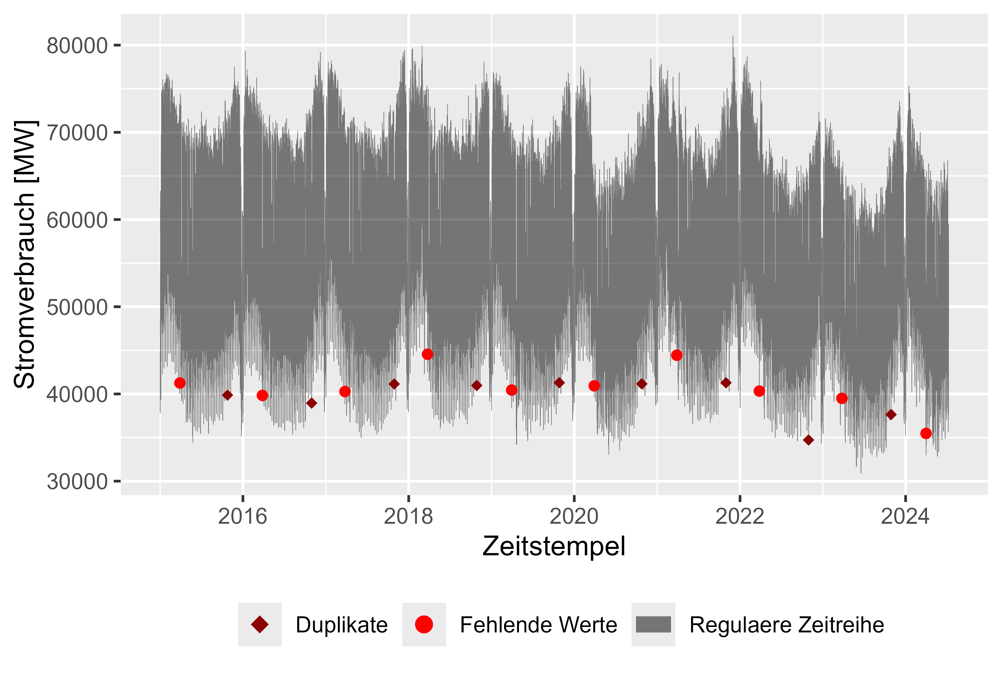 Figure 1 Raw power consum
local_name_colors <- c(
  "Christi Himmelfahrt" = palette()[2],
  "Erster Weihnachtstag" = palette()[2],
  "Karfreitag" = palette()[2],
  "Neujahr" = palette()[2],
  "Ostermontag" = palette()[2],
  "Pfingstmontag" = palette()[2],
  "Reformationstag" = palette()[2],
  "Tag der Arbeit" = palette()[2],
  "Tag der Deutschen Einheit" = palette()[2],
  "Zweiter Weihnachtstag" = palette()[2],
  "Regulärer Tag" = palette()[1]
)


week_colors <- c(
  "Mo" = palette()[1],
  "Di" = palette()[1],
  "Mi" = palette()[1],
  "Do" = palette()[1],
  "Fr" = palette()[1],
  "Sa" = palette()[2],
  "So" = palette()[2]
)

working_colors <- c("1" = "#2E9FDF", "0" = "#FC4E07")

whw_colors <- c(
  "FeiertagnKein Wochenende" = "black",
  "Kein FeiertagnKein Wochenende" = "red",
  "Kein FeiertagnWochenende" = "orange",
  "FeiertagnWochenende" = "blue"
)

p <- cleaned_power_consum |>
    gg_tsdisplay(PowerConsum, plot_type = "partial", lag = 100)

ggsave(
  "plots/power_consum_acf_pacf.png",
  plot = p,
  width = 5.5,
  height = 3.7,
  dpi = 600
)

plot_calculated_features(
  cleaned_power_consum = cleaned_power_consum,
  file_name = "plots/MinLastOneDay.png",
  x = "MinLastOneDay",
  y = "PowerConsum",
  x_label = "Minimaler Stromverbrauch vom letzten Tag [MW]",
  y_label = "Stromverbrauch [MW]"
)

plot_calculated_features(
  cleaned_power_consum = cleaned_power_consum,
  file_name = "plots/MaxLastOneDay.png",
  x = "MaxLastOneDay",
  y = "PowerConsum",
  x_label = "Maximaler Stromverbrauch vom letzten Tag [MW]",
  y_label = "Stromverbrauch [MW]"
)

plot_calculated_features(
  cleaned_power_consum = cleaned_power_consum,
  file_name = "plots/MeanLastWeek.png",
  x = "MeanLastWeek",
  y = "PowerConsum",
  x_label = "Durchschnittlicher Stromverbrauch der letzten 7 Tage [MW]",
  y_label = "Stromverbrauch [MW]"
)


plot_calculated_features(
  cleaned_power_consum = cleaned_power_consum,
  file_name = "plots/MeanLastTwoDays.png",
  x = "MeanLastTwoDays",
  y = "PowerConsum",
  x_label = "Durchschnittlicher Stromverbrauch der letzten 2 Tage [MW]",
  y_label = "Stromverbrauch [MW]"
)

plot_histogram_by_group(
  cleaned_power_consum,
  group_name = "WorkdayHolidayWeekend",
  file_name = "plots\workday_holiday_weekend_histogram.png",
  colors = whw_colors,
  x="PowerConsum",
  x_label = "Stromverbrauch [MW]",
  y_label = "Häufigkeit",
  name_0 = "Wochenende oder Feiertage",
  name_1 = "Werktag"
)


plot_histogram_by_group(
  cleaned_power_consum,
  group_name = "WorkDay",
  file_name = "plots\workday_histogram.png",
  colors = working_colors,
  x="PowerConsum",
  x_label = "Stromverbrauch [MW]",
  y_label = "Häufigkeit",
  name_0 = "Wochenende oder Feiertage",
  name_1 = "Werktag"
)

plot_histogram_by_group(
  cleaned_power_consum,
  group_name = "Holiday",
  file_name = "plots\holiday_histogram.png",
  colors = working_colors,
  x="PowerConsum",
  x_label = "Stromverbrauch [MW]",
  y_label = "Häufigkeit",
  name_0 = "Werktag oder Wochenende",
  name_1 = "Feiertag"
)

plot_histogram_by_group(
  cleaned_power_consum,
  group_name = "HolidayAndWorkDay",
  file_name = "plots\holiday_workday_histogram.png",
  colors = working_colors,
  x="PowerConsum",
  x_label = "Stromverbrauch [MW]",
  y_label = "Häufigkeit",
  name_0 = "Wochenende oder Werktag",
  name_1 = "Feiertag am Werktag"
)

plot_by_group(
  cleaned_power_consum,
  group_name = "HolidayName",
  file_name = "plots\holiday_boxplot.png",
  colors = local_name_colors,
  title = "Übersicht der einzelnen Feiertage",
  y="PowerConsum",
  y_label="Stromverbrauch [MW]",
  x_label="Jahre"
)

plot_by_group(
  cleaned_power_consum,
  group_name = "Weekday",
  file_name = "plots\weekday_boxplot.png",
  colors = week_colors,
  title = "Übersicht der einzelnen Wochentage",
  y = "PowerConsum",
  y_label="Stromverbrauch [MW]",
  x_label="Jahre"
)

plot_by_group(
  cleaned_power_consum,
  group_name = "WorkDay",
  file_name = "plots\workday_boxplot.png",
  colors = working_colors,
  title = "Übersicht, ob Feiertag (FALSE) oder Werktag (TRUE)",
  y = "PowerConsum",
  y_label="Stromverbrauch [MW]",
  x_label="Jahre"
)


plot_by_column(
  df = cleaned_power_consum,
  x = "Hour",
  y = "PowerConsum",
  x_label = "Stunden",
  y_label = "Stromverbrauch [MW]",
  file_name = "plots\hour_boxplot.png",
  title = "Übersicht der einzelnen Stunden"
)

plot_by_column(
  df = cleaned_power_consum,
  x = "Month",
  y = "PowerConsum",
  x_label = "Monate",
  y_label = "Stromverbrauch [MW]",
  file_name = "plots\month_boxplot.png",
  title = "Übersicht der einzelnen Monate"
)

plot_by_column(
  df = cleaned_power_consum,
  x = "Week",
  y = "PowerConsum",
  x_label = "Woche",
  y_label = "Stromverbrauch [MW]",
  file_name = "plots\week_boxplot.png",
  title = "Übersicht der einzelnen Wochen"
)

plot_by_column(
  df = cleaned_power_consum,
  x = "Year",
  y = "PowerConsum",
  x_label = "Jahr",
  y_label = "Stromverbrauch [MW]",
  file_name = "plots\year_boxplot.png",
  title = "Übersicht der einzelnen Jahre"
)

plot_year_month_week_day(
  df=cleaned_power_consum,
  date_column="DateIndex",
  y="PowerConsum",
  from_year=2015,
  to_year=2024,
  from_week=0,
  to_week=53,
  year_for_week=2018,
  from_day=1,
  to_day=30,
  month_for_day=4,
  year_for_day=2018,
  from_month=1,
  to_month=12,
  year_for_month=2018,
  holiday="Holiday",
  day_of_week = "Weekday"
)
Following sections will go more and more in detail of the data. We will start here with the yearly representation.
Figure 2 is yearly representation of the years 2015-2024. We can notice here, that in the beginning of the year there is an increase of power consum and in the end of the year there is a decrease (Christmas, New-year). Overall looks like a smile-shape or a bow.
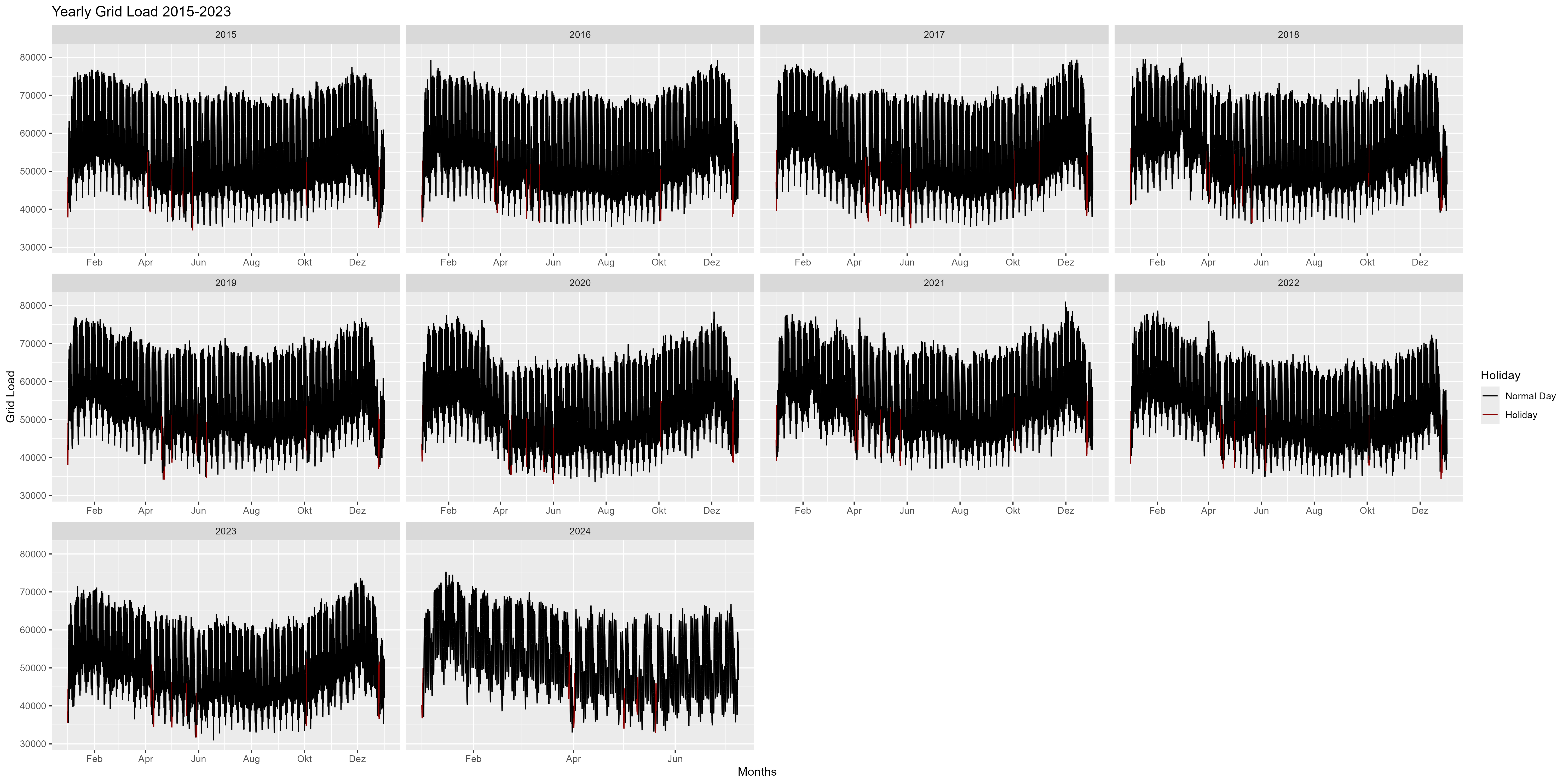 Figure 2 Power consum, every year as a single facet
Let's try to aggregate all the years and split them into weeks.
The boxplots in Figure 3 combine all years. We can see the pattern in more detail.
Beginning and the end of a year is represented in red and shows a decrease from the regular "smile-shape".
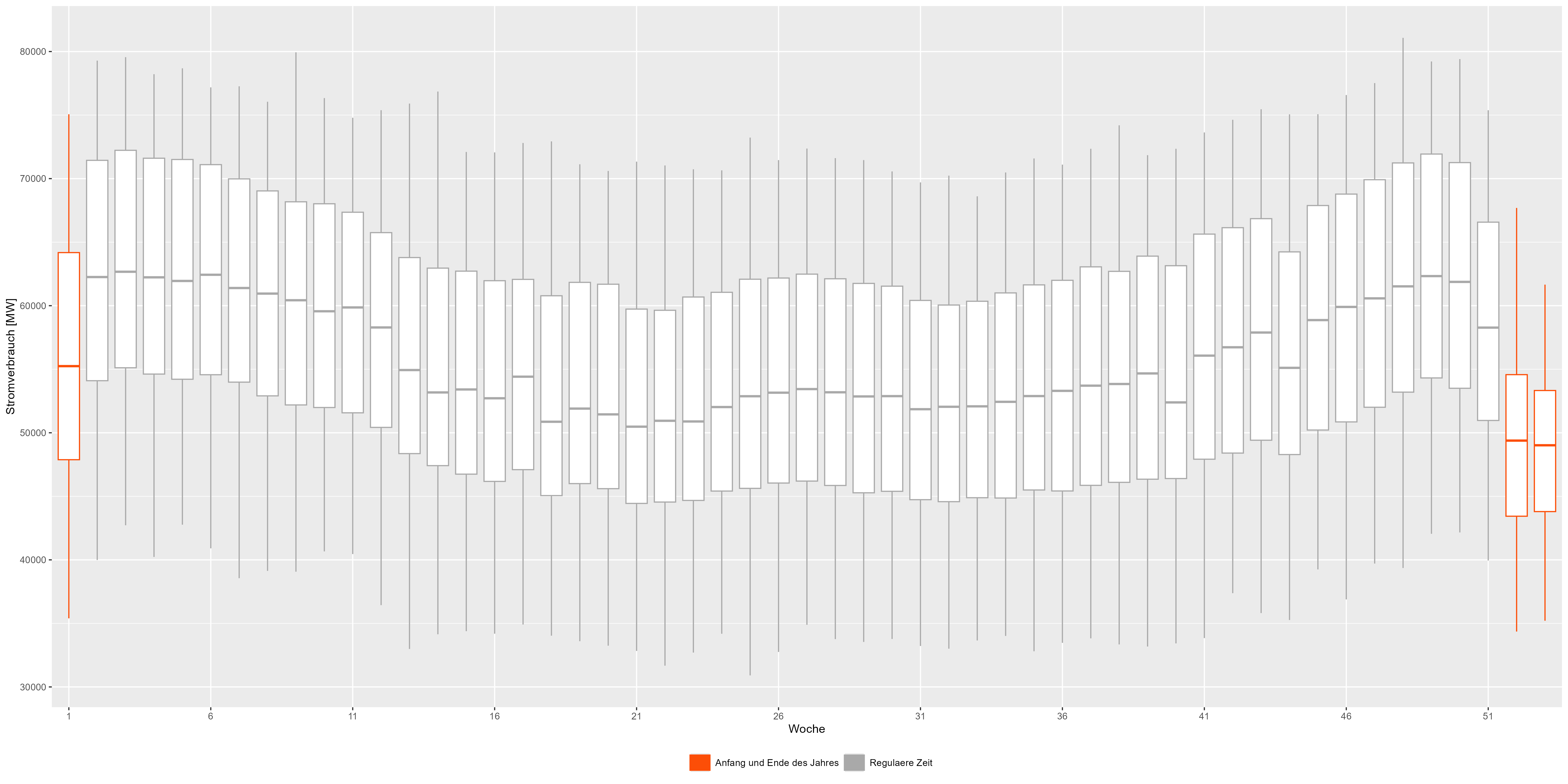 Figure 3 Power consum weekly aggregated data
Let's go more in detail and look into the year 2018 for example. Figure 4 is the monthly representation of the year 2018. Here we can observe in more detail the end of the year. Around 24th December, there is a decrease of power consum. Also notable here are the weekends and the holidays (red). A decrease for all weekends and for all holidays.
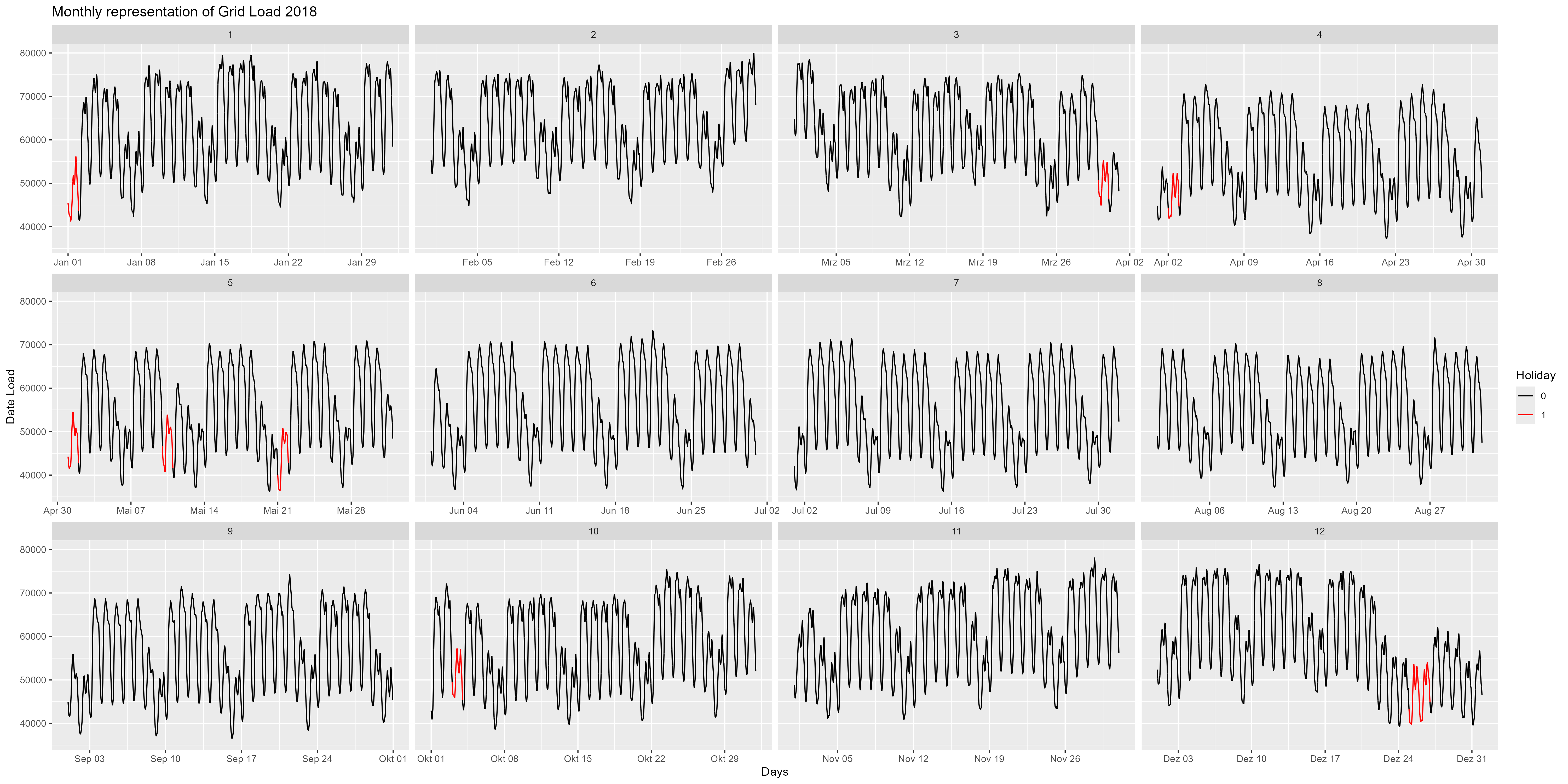 Figure 4 Power consum, every month as a single facet
We could go even further and check out the hourly representation of the data. Figure 5 shows the aggregated boxplot for every hour. There is also a decrease in the nighttime (21:00-06:00) and an increase in the daytime / work-time (06:00-21:00). Also a pattern that needs to be included in the model.
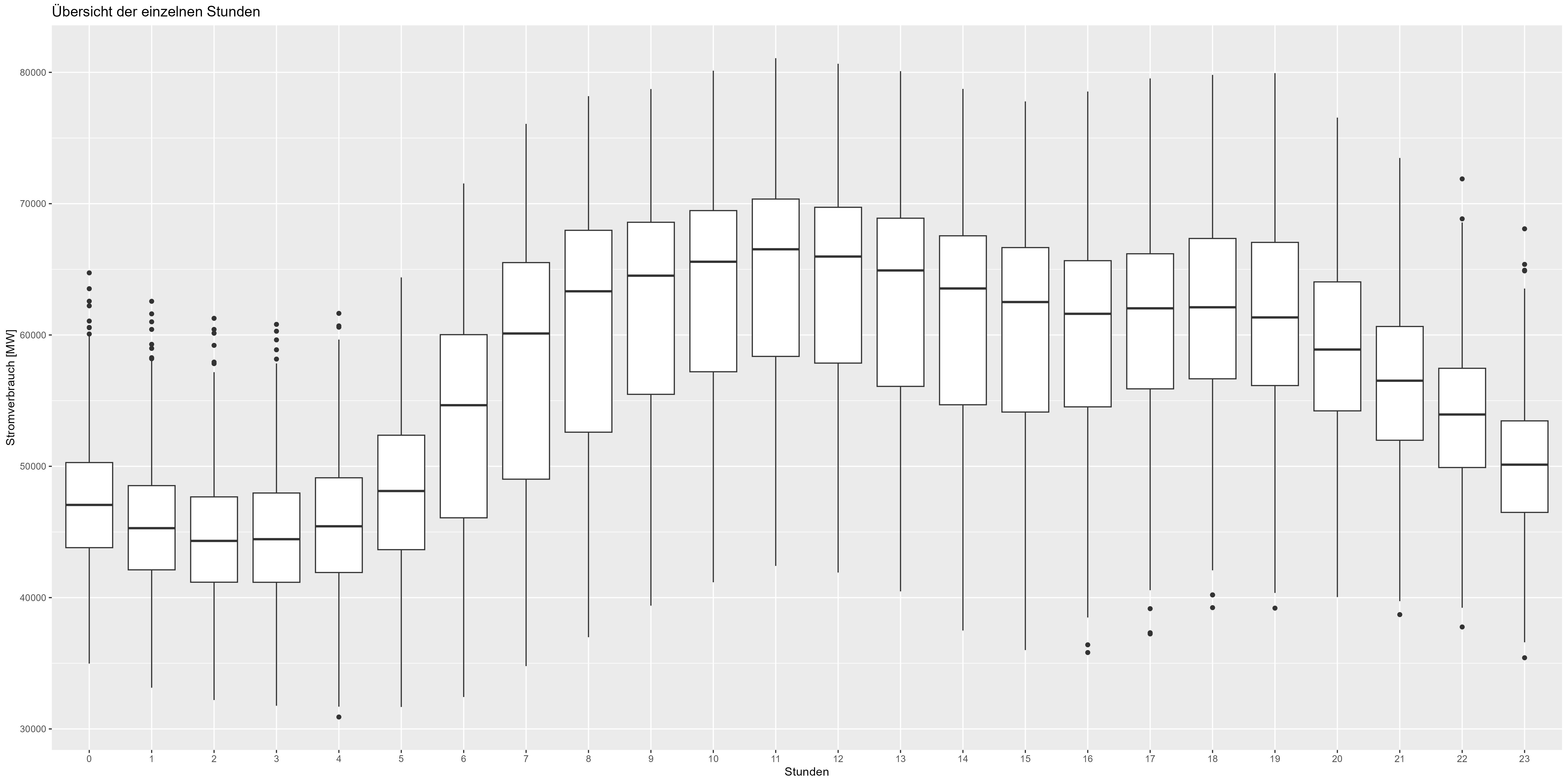 Figure 5 Power consum hourly aggregated data
Let's talk about weekdays. As assumed in the weekend power consum decreases. "Durchschnitt" is the mean. Figure 6 shows all weekdays (aggregated) over the years. There is a decrease of ~10.000 MW for weekends.
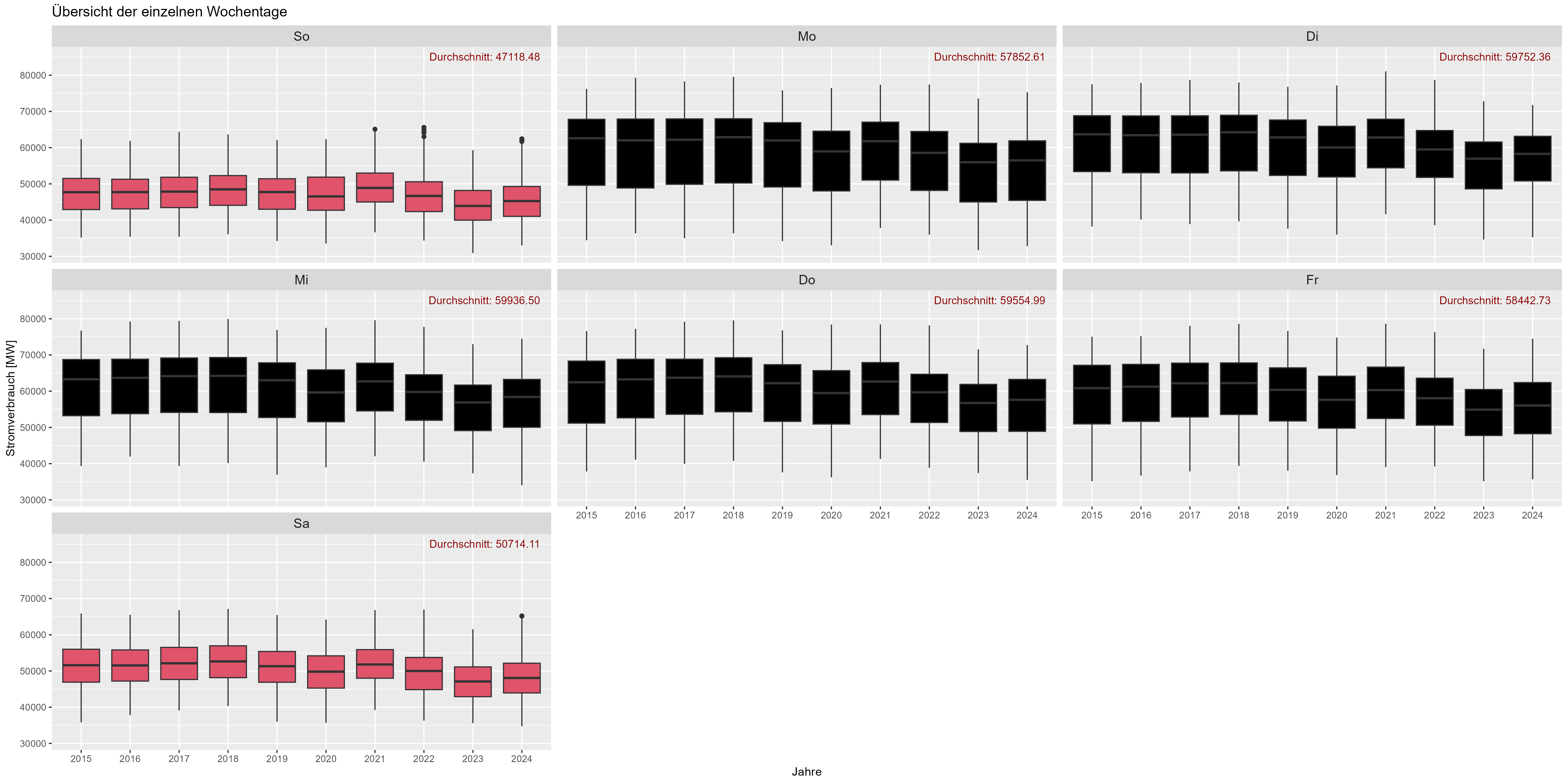 Figure 6 Power consum "day-of-week-effect"
Figure 8 shows the holiday effect. "Durchschnitt" is the mean power consum over years. There is a significant increase of power consum for "Working-Days" (darkgrey) compared with holidays (red). We could assume here that holidays acts like weekends for the Power-Consum".
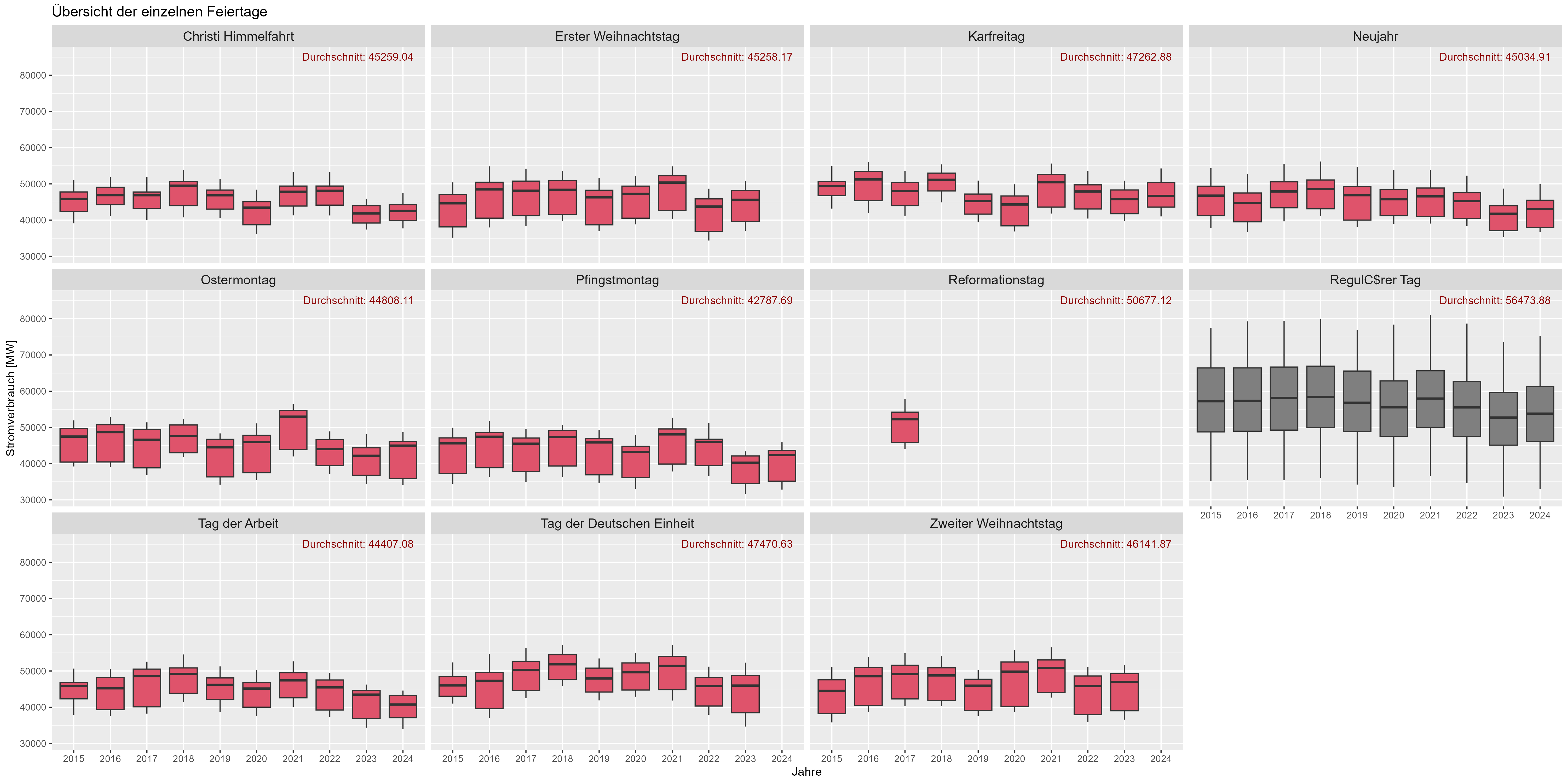 Figure 6 Power consum "holiday-effect"
Figure 7 represent different behaviours for different days. There are 4 categories. "Feiertag Kein Wochenende" means it is a holiday, but not a weekend. "Feiertag Wochenende" means it is a holiday and a weekend. "Kein Feiertag Kein Wochenende" means it is a regular working day and "Kein Feiertag Wochenende" means it is just the weekend. We can observe similar distributions for not regular working days as assumed.
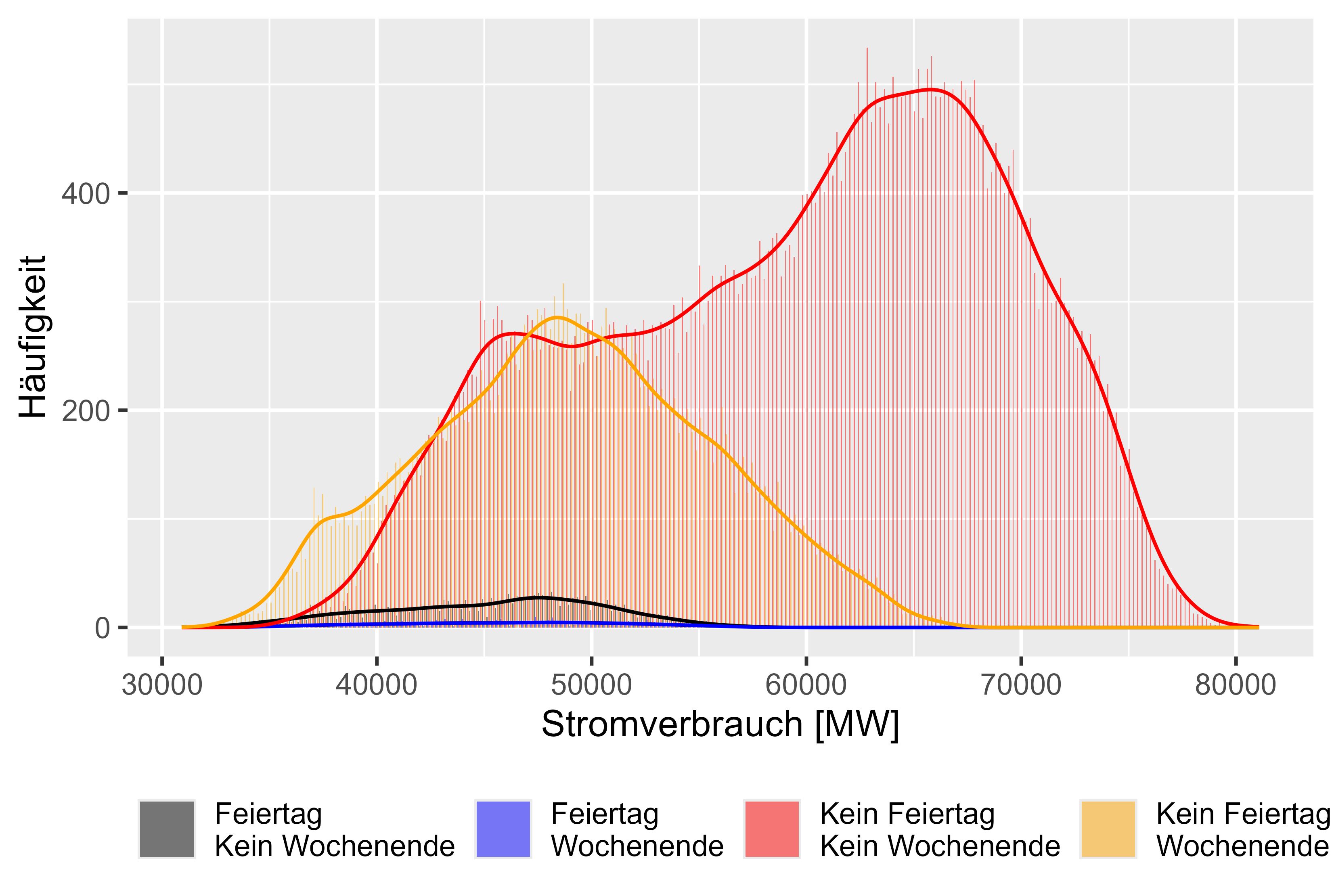 Figure 7 Power consum "Different-Effects" compared
Lagged values like MeanLastTwoDays, MeanLastWeek, MaxLastOneDay and MinLastOneDay are generated features.
Similar as discussed in DOI: 10.1109/TPWRS.2011.2162082 - Short-Term Load Forecasting Based on a Semi-Parametric Additive Model
Figures 8-11 (red are not working days) represent this lagged values against the actual power consum.
There is a light correlation for this generated features.
# Check Correlation
cor <- cor(cleaned_power_consum[sapply(cleaned_power_consum, is.numeric)], method = c("pearson", "kendall", "spearman"), use = "complete.obs")
| Feature | Correlation with PowerConsum |
|---|---|
| HolidaySmoothed | -0.556194 |
| MeanLastWeek | 0.389044 |
| MeanLastTwoDays | 0.201253 |
| MaxLastOneDay | 0.320193 |
| MinLastOneDay | 0.348583 |
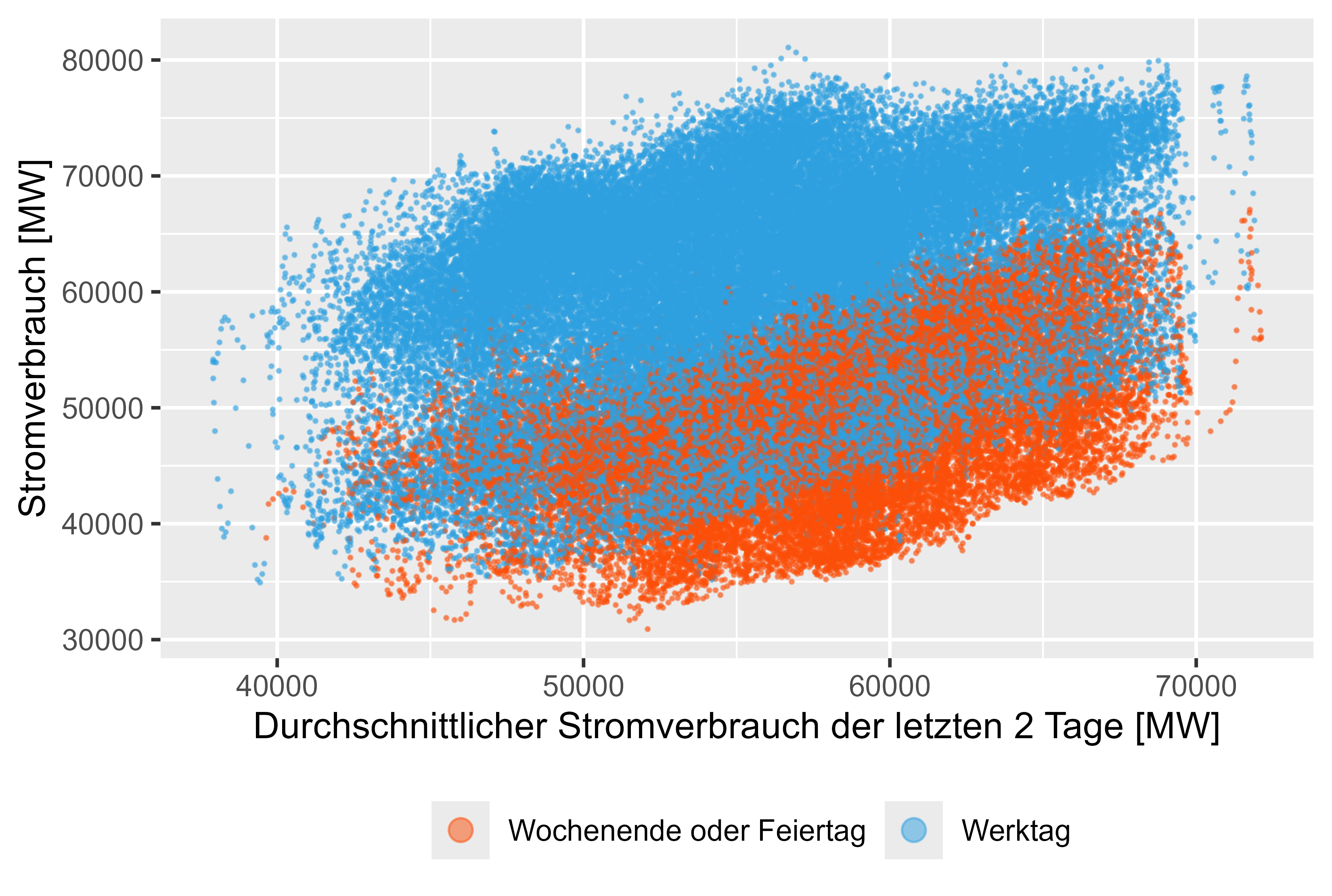 Figure 8 Power-Consum - MeanLastTwoDays
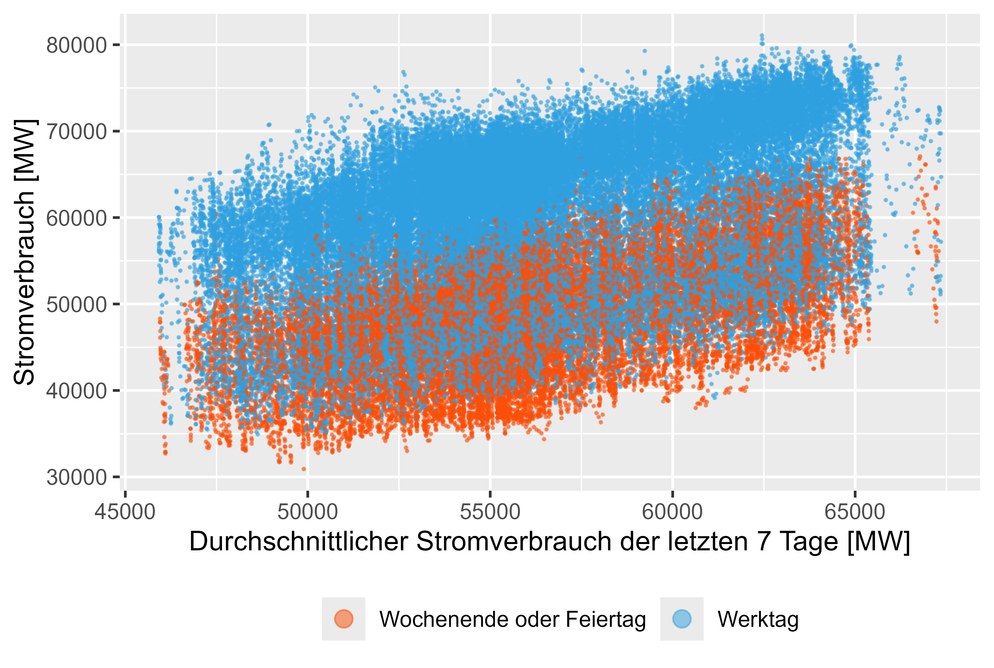 Figure 9 Power-Consum - MeanLastWeek
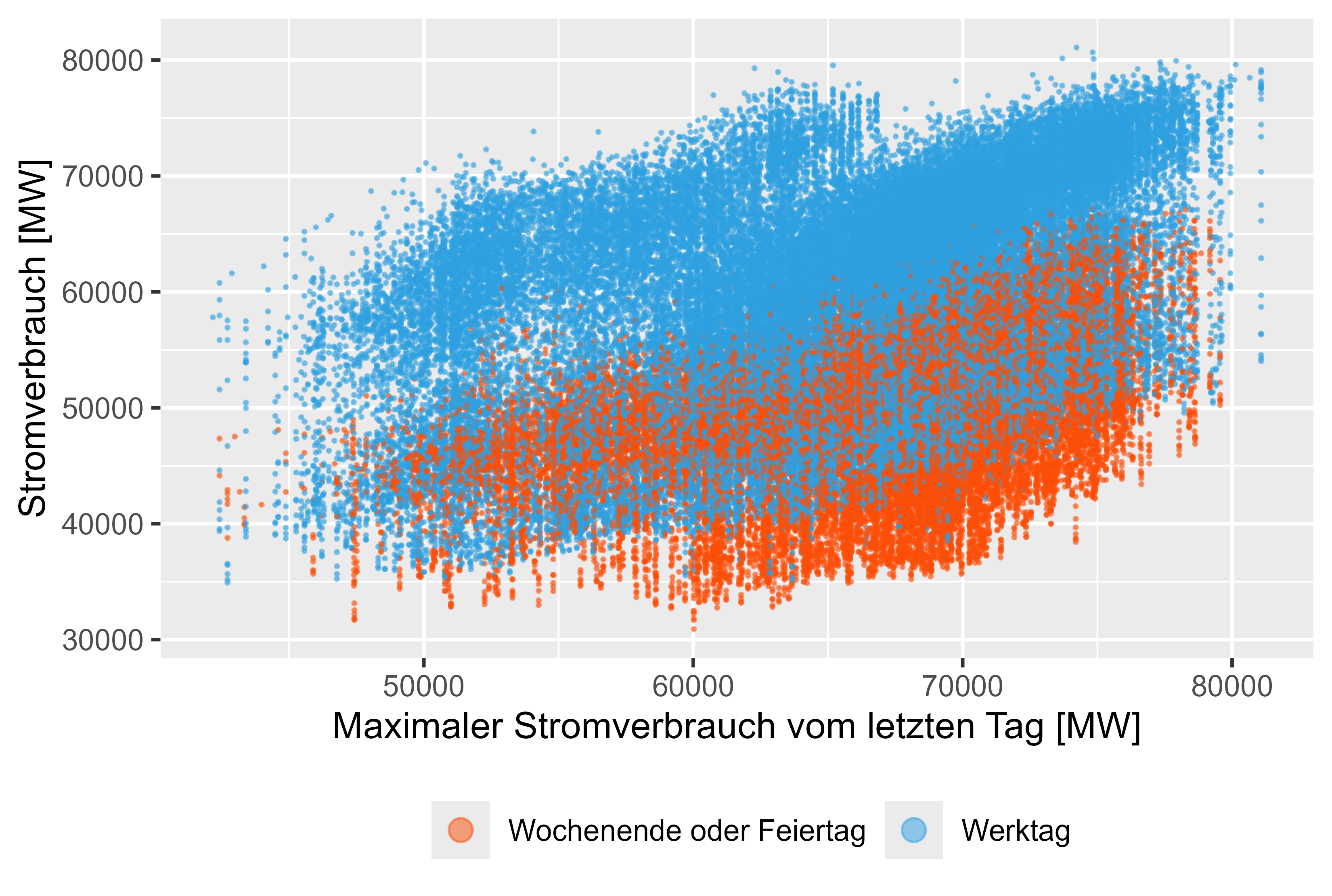 Figure 10 Power-Consum - MaxLastOneDay
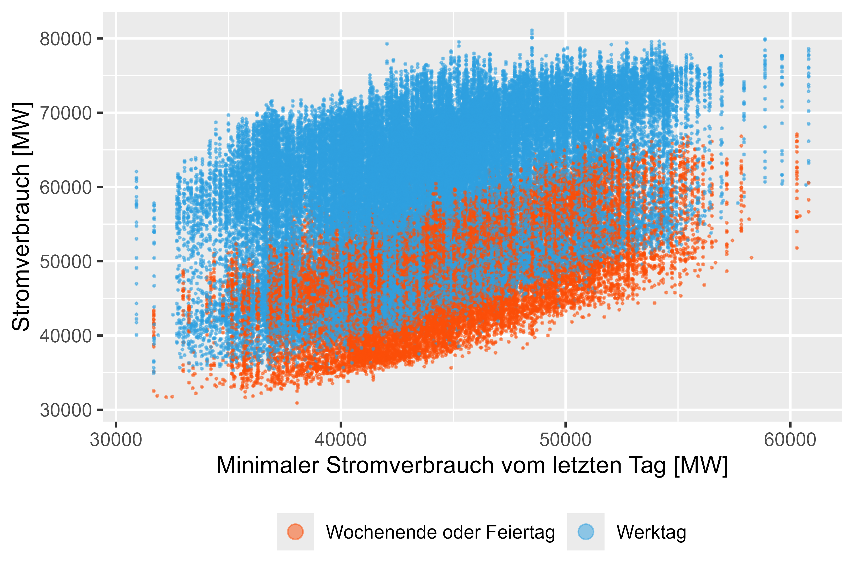 Figure 11 Power-Consum - MinLastOneDay
There is a complex seasonality. For the hourly resolution there is a yearly, weekly and a daily seasonality. Which needs to be tracked by the model. The solution here is as discussed in Forecasting: Principles and Practice Chapter 12.1 Complex seasonality to use fourier-terms to represent and assemble via cos() and sin() the complex seasonality.
We can take a small view on the ACF and PACF plot, there are few significant spikes, but it is just the representation of 96 lagged values. If we take the ~9000 lagged Observations for a year there would be a complex seasonality. That's why it is easier to go with fourier-term. It also didn't work well just finding PDQ and pdq components by
ARIMA(...
stepwise=FALSE,
greedy=FALSE,
approx=FALSE)
itself. Also the training time increases dramatically without the fourier-terms.
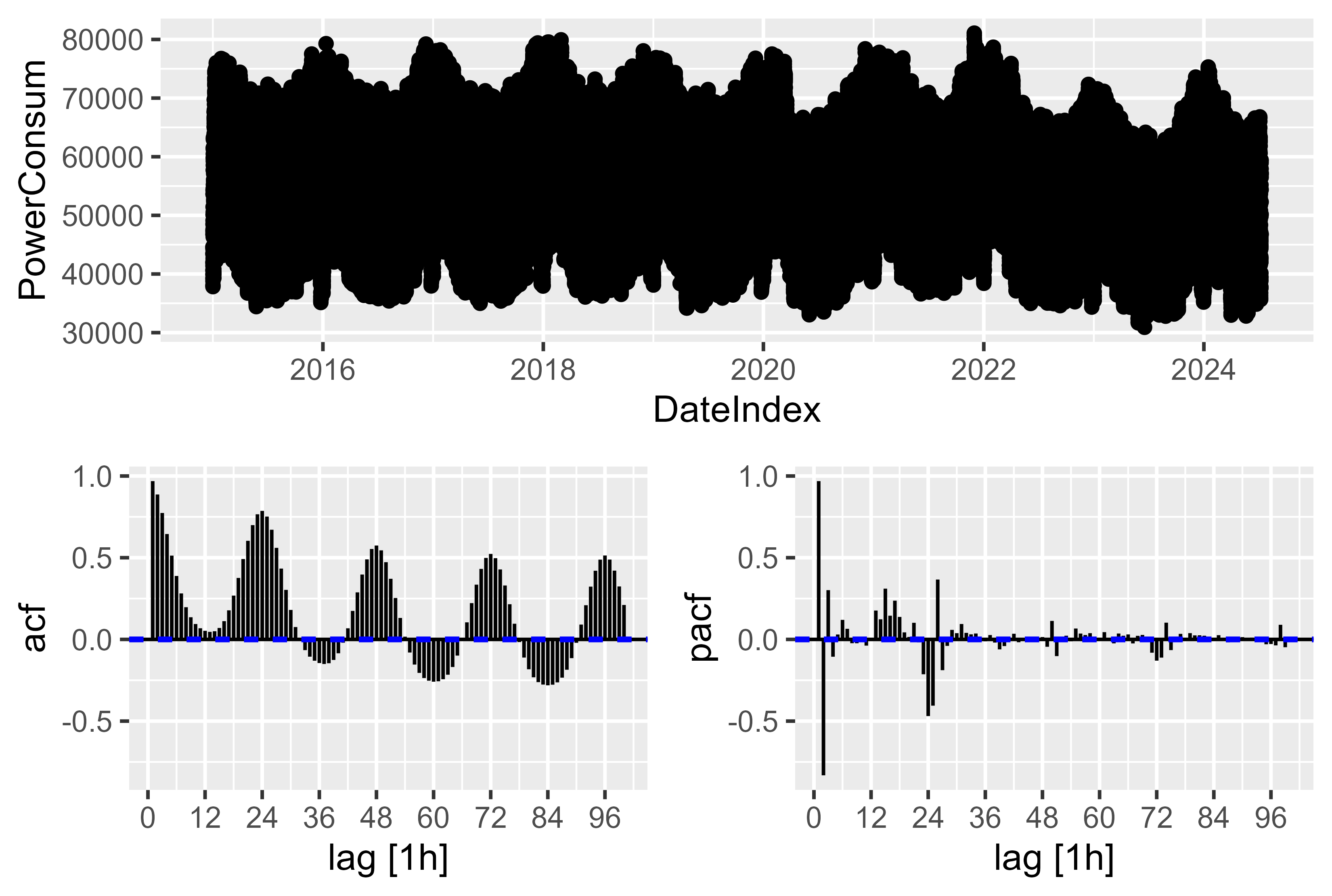 Figure 12 Power-Consum - ACF PACF Plot of raw power consum
Best feature combination found in this work are:
To compare the models we use metrics MAE and MAPE. SMARD is the model of "Bundesnetzagentur" from the SMARD page. Prophet model was also tried out, performed solid, but not good enough.
The SMARD forecasted values reached a MAPE of 3.6%. <- NOT IN THIS STUDY.
Training-Data:
The best model found so far war LHM + DHR (linear-harmonic-model + dynamic-harmonic-regression)
The idea is to ensemble a linear model with ARIMA model. Because it was hard for ARIMA model to deal with dummy-variables for Holidays. So the ensembled model helped out.
train_power_consum <- cleaned_power_consum |>
    filter(year(DateIndex) > 2020 & (year(DateIndex) < 2024))

generate_models(model_name = "model/mean_naive_drift",
                train_power_consum = train_power_consum)

train_power_consum_v5 <- train_power_consum |>
  mutate(HolidaySmoothed = Holiday + sin(2 * pi * (as.numeric(Hour)+1) / 24))

holiday_effect_model <- lm(
  PowerConsum ~
    HolidaySmoothed,
  data = train_power_consum_v5
)

saveRDS(holiday_effect_model, file = "ensemble_model/version_5/holiday_effect_2021_2023.rds")

train_power_consum_v5$Residuals <- residuals(holiday_effect_model)

fit <- train_power_consum_v5 |>
  model(
    ARIMA = ARIMA(Residuals ~
                    PDQ(0,0,0)
                  + pdq(d=0)
                  + MeanLastWeek
                  + WorkDay
                  + EndOfTheYear # new
                  + FirstWeekOfTheYear # new
                  + MeanLastTwoDays
                  + MaxLastOneDay
                  + MinLastOneDay
                  + fourier(period = "day", K = 6)
                  + fourier(period = "week", K = 7)
                  + fourier(period = "year", K = 3)
    )
  )

saveRDS(fit, file = "ensemble_model/version_5/arima_2021_2023.rds")
We could visualize the effect and how the model works. Figure 13 shows the idea behind this model. First of all we fit the LHM model and calculate the residuals. Train the DHR model by the residuals and sum up both. It's kinda mirror on the LHM and push the values back to the top.
For the LHM model we use here a simple approach a sinus curve that repeats every 24 hours and decrease or increase on Holidays or workdays.
By forecasting LHM on new data we can forecast the residuals for new data. Residuals + LHM shift the values back to the "correct" position.
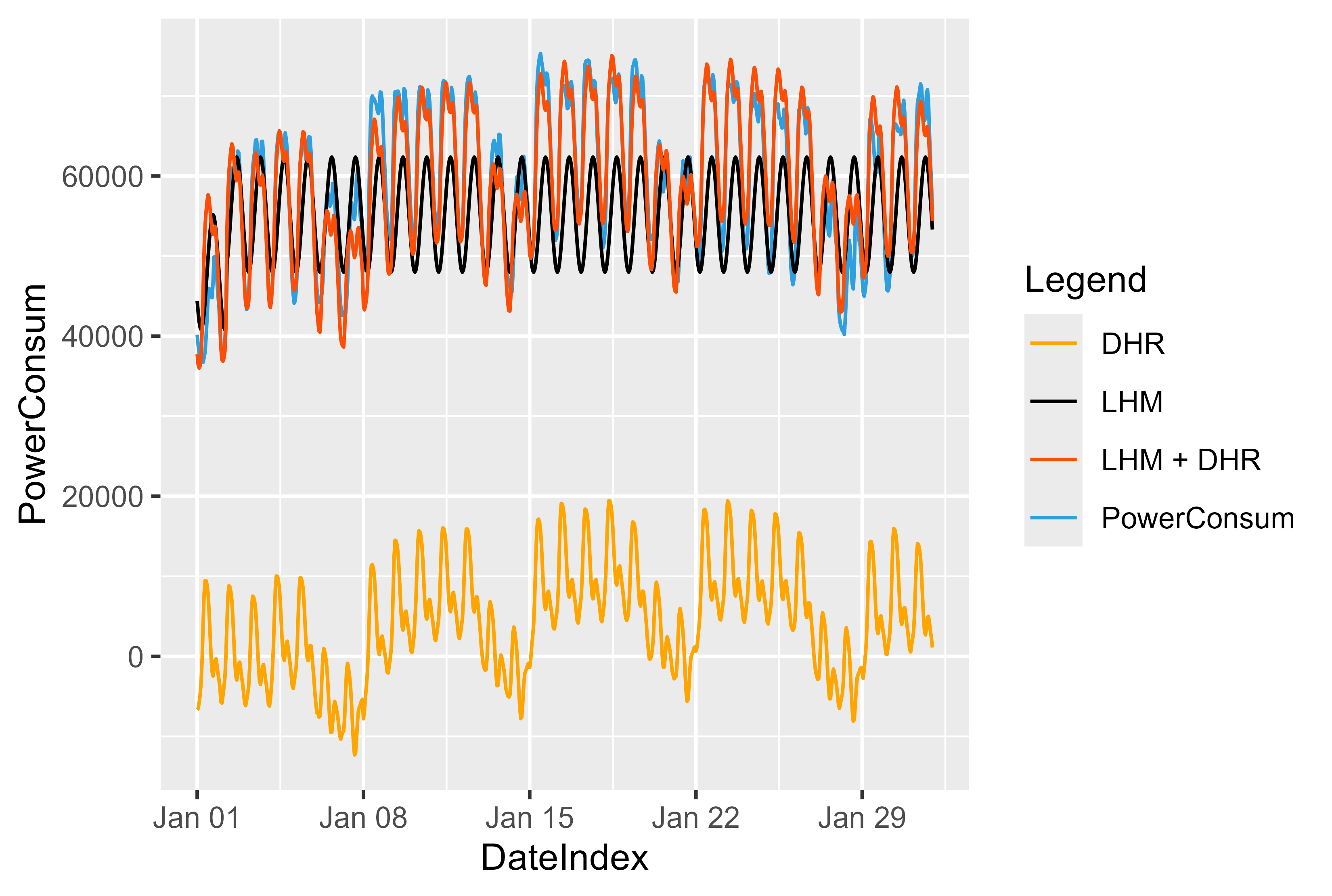 Figure 13 LHM + DHR Model representation
ensembled_fc <- load_ensembled_models(
  days_to_forecast = 40,
  months_to_forecast = 6,
  year_to_forecast = 2024,
  starting_month = 1,
  real_data = cleaned_power_consum,
  smard_fc = cleaned_smard_pred,
  model_path = "ensemble_model"
)
all_forecasts_ensembled <- ensembled_fc$all_forecasts
raw_fc_ensembled <- ensembled_fc$raw_forecasts

fc <- load_all_model_results(
  days_to_forecast = 40,
  months_to_forecast = 6,
  year_to_forecast = 2024,
  starting_month = 1,
  smard_fc = cleaned_smard_pred,
  real_data = cleaned_power_consum
)

all_forecasts <- fc$combined_forecasts
raw_fc <- fc$raw_forecasts


metric_results <- calculate_metrics(fc_data = all_forecasts, fc_data_ensembled=all_forecasts_ensembled)

# Plot best Model for single Models
name_of_best_model_for_single_model <- plot_forecast(
  all_forecasts = all_forecasts,
  metric_results = metric_results,
  cleaned_power_consum = cleaned_power_consum,
  raw_fc = raw_fc,
  month_to_plot = 1,
  days_to_plot = 40
)

# Plot best Model for ensembled Models
name_of_best_model_ensembled <- plot_forecast_ensembled(
  all_forecasts = all_forecasts_ensembled,
  metric_results = metric_results,
  cleaned_power_consum = cleaned_power_consum,
  month_to_plot = 1,
  days_to_plot = 40
)

# Residuals Compared with SMARD
plot_compare_with_smard(
  all_forecasts = all_forecasts_ensembled,
  name_of_best_model = name_of_best_model_ensembled
  )


# LHM DHM representation
plot_representation_of_lhm_dhm_components(path_dhm = "ensemble_model/version_5/arima_2021_2023.rds",
                                          path_lhm = "ensemble_model/version_5/holiday_effect_2021_2023.rds",
                                          from_month = 1,
                                          to_month = 1,
                                          raw_fc_ensembled = raw_fc_ensembled)
A solid score of MAPE 3.8% for version_5 (LHM + DHR Model).
Lets's take a deeper look if we would use just the ARIMA model (arima_14). Figure 14 represents the results for this model. We can see the holidays (orange), Weekend (red) and regular day (blue). There are significant outliers for the holidays, even though there was a dummy-variable for the ARIMA model it couldn't catch the holidays correctly.
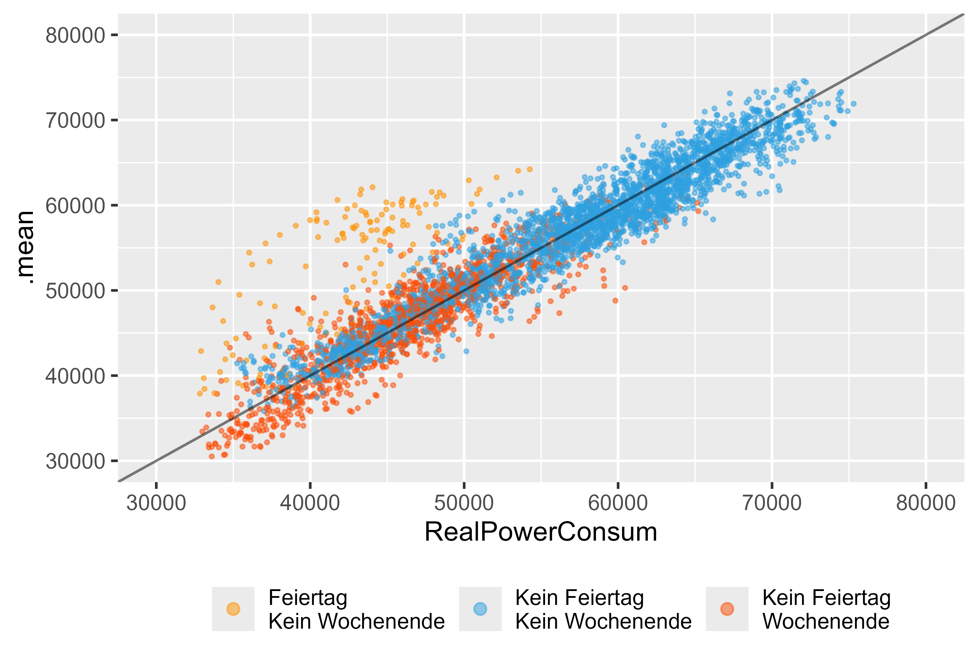 Figure 14 Forecast vs Actual Values ARIMA (DHR, arima_14), as a single model
On the other hand the LHM + DHR Model shows a better performence for the holidays. Figure 15 represents it.
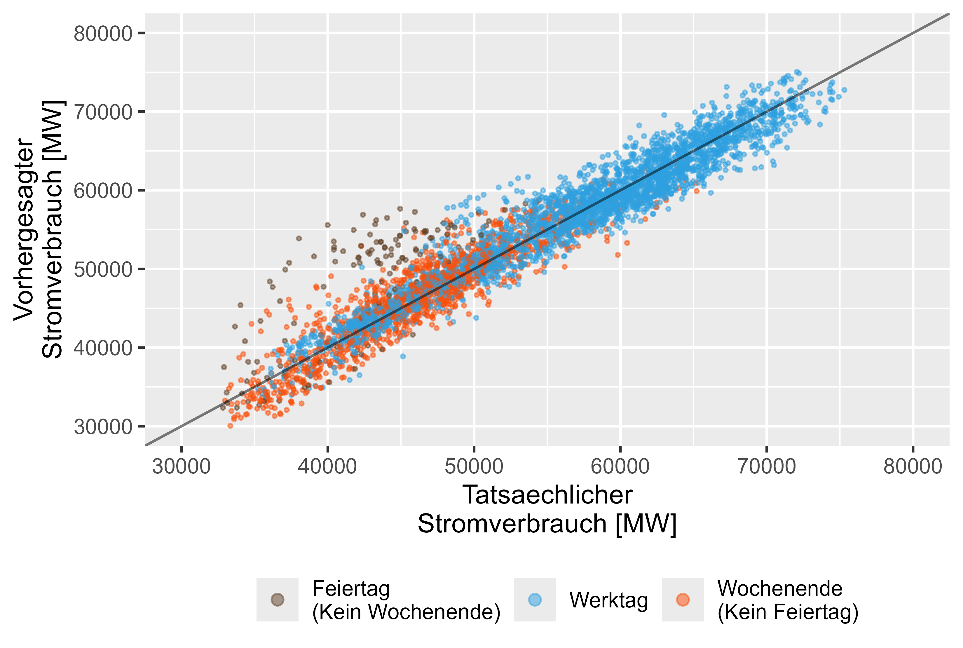 Figure 15 Forecast vs Actual Values LHM + DHR, ensembled model
Figure 16 shows the forecast for january 2024. It looks reasonable.
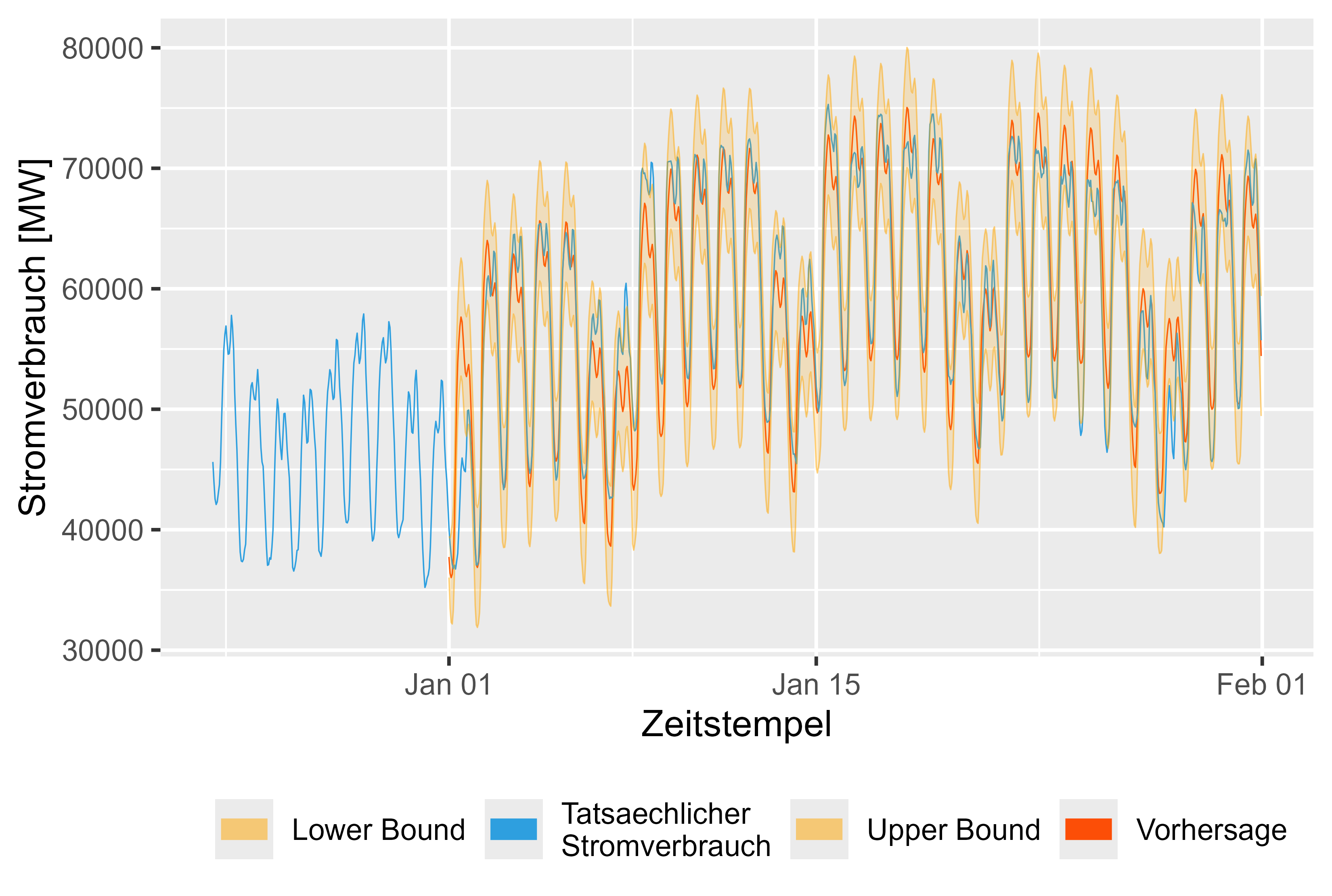 Figure 16 Forecast vs Actual Values LHM + DHR for january 2024
Also the Residuals for the model compared with the SMARD model looks fine. There are few spikes, that could be significant and may be prepared better by modeling. But overall a solid result.
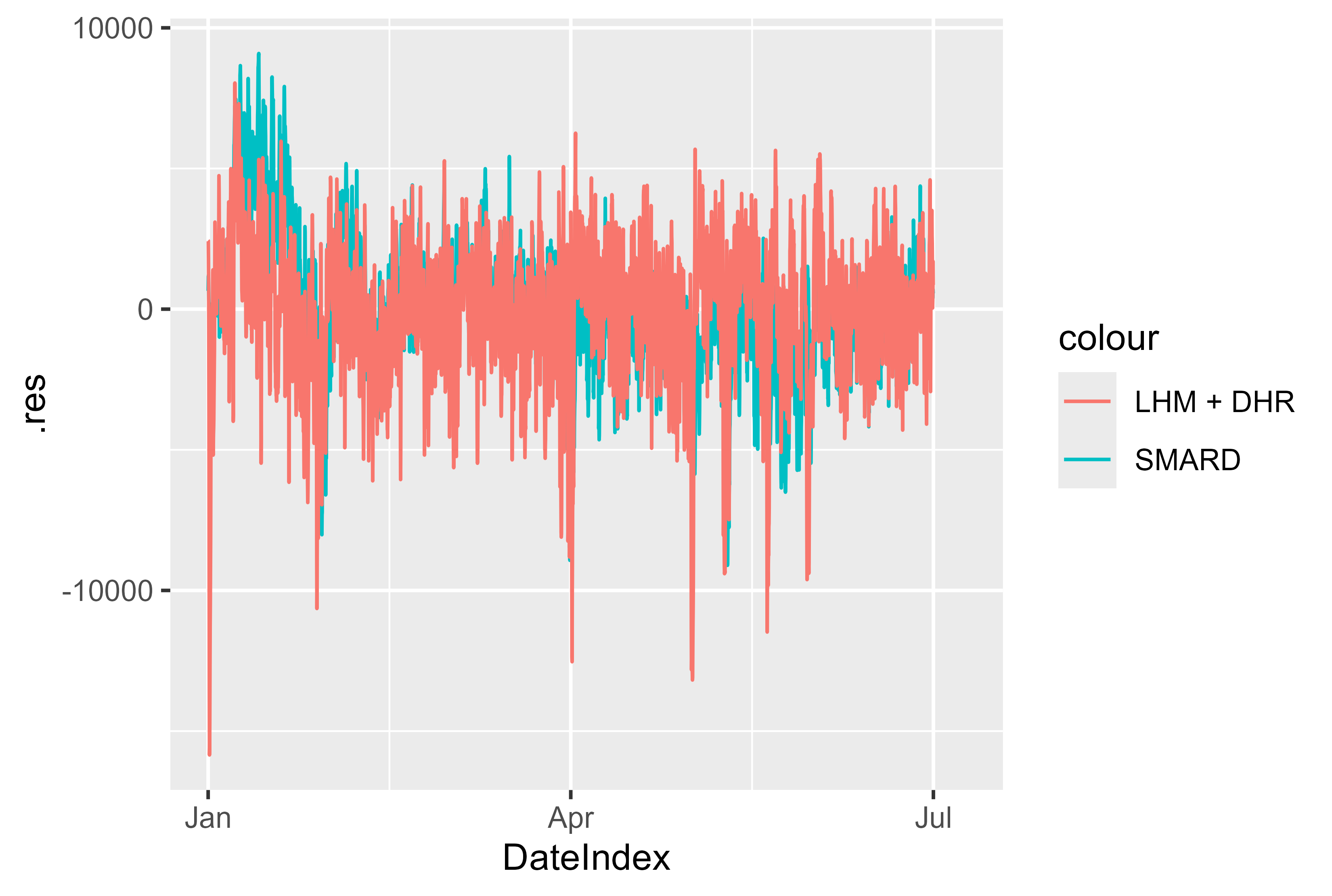 Figure 17 Residuals LHM + DHR for january - july 2024
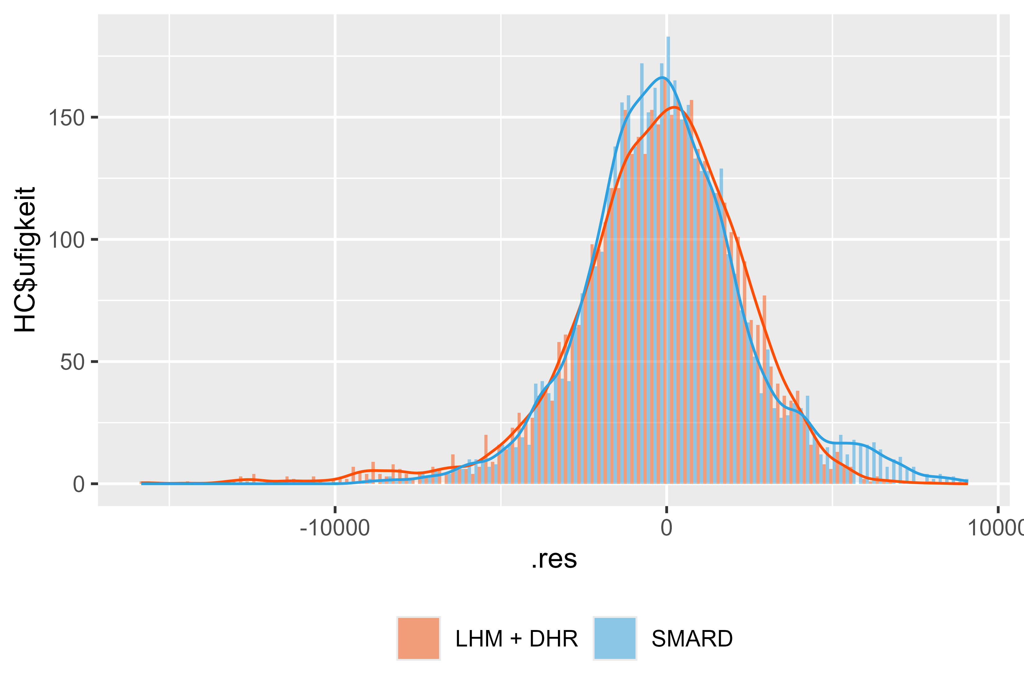 Figure 18 Residuals LHM + DHR for january - july 2024
| Index | Model Name | RMSE | MAPE | MAE | Ensembled |
|---|---|---|---|---|---|
| 2 | RealObservations | 0.000 | 0.000000 | 0.000 | TRUE |
| 3 | SMARD | 2480.693 | 3.602140 | 1869.466 | FALSE |
| 4 | SMARD | 2480.693 | 3.602140 | 1869.466 | TRUE |
| 5 | version_5 | 2626.807 | 3.816012 | 1937.670 | TRUE |
| 6 | version_0 | 2613.258 | 3.846888 | 1946.314 | TRUE |
| 7 | version_7 | 2770.359 | 4.107272 | 2076.045 | TRUE |
| 8 | version_8 | 2775.441 | 4.146788 | 2091.153 | TRUE |
| 9 | version_9 | 2887.179 | 4.177841 | 2100.381 | TRUE |
| 10 | version_6 | 2906.242 | 4.216517 | 2142.092 | TRUE |
| 11 | arima_14_2021_2023.rds | 3208.735 | 4.389492 | 2207.395 | FALSE |
| 12 | arima_18_2021_2023.rds | 3208.735 | 4.389492 | 2207.395 | FALSE |
| 13 | version_4 | 2875.929 | 4.535388 | 2255.645 | TRUE |
| 14 | version_2 | 2905.990 | 4.580770 | 2279.624 | TRUE |
| 15 | arima_9_2021_2023.rds | 3267.160 | 4.611857 | 2302.918 | FALSE |
| 16 | arima_2_2021_2023.rds | 3251.390 | 4.614028 | 2301.447 | FALSE |
| 17 | arima_4_2021_2023.rds | 3251.390 | 4.614028 | 2301.447 | FALSE |
| 18 | arima_5_2021_2023.rds | 3251.390 | 4.614028 | 2301.447 | FALSE |
| 19 | arima_13_2021_2023.rds | 3283.745 | 4.619636 | 2307.415 | FALSE |
| 20 | arima_10_2021_2023.rds | 3265.913 | 4.625508 | 2314.395 | FALSE |
| 21 | arima_0_2021_2023.rds | 3269.009 | 4.645944 | 2317.138 | FALSE |
| 22 | arima_17_2021_2023.rds | 3269.009 | 4.645944 | 2317.138 | FALSE |
| 23 | arima_16_2021_2023.rds | 3298.902 | 4.673116 | 2334.857 | FALSE |
| 24 | arima_1_2021_2023.rds | 3312.429 | 4.696342 | 2340.193 | FALSE |
| 24 | prophet_0_2021_2023.rds | 3044.849 | 4.711527 | 2435.572 | FALSE |
| 25 | arima_8_2021_2023.rds | 3332.217 | 4.716612 | 2358.085 | FALSE |
| 26 | arima_11_2021_2023.rds | 3358.020 | 4.758970 | 2388.791 | FALSE |
| 27 | arima_12_2021_2023.rds | 3430.191 | 5.022772 | 2495.067 | FALSE |
| 28 | arima_7_2021_2023.rds | 3475.671 | 5.049287 | 2510.903 | FALSE |
| 29 | version_3 | 3546.729 | 5.064654 | 2570.530 | TRUE |
| 30 | arima_15_2021_2023.rds | 3734.584 | 5.165147 | 2606.661 | FALSE |
| 31 | arima_6_2021_2023.rds | 3748.583 | 5.375326 | 2723.837 | FALSE |
| 32 | version_1 | 4495.568 | 6.483477 | 3229.647 | TRUE |
| 33 | arima_3_2021_2023.rds | 4558.982 | 6.953247 | 3453.387 | FALSE |
| 34 | tslm_0_2021_2023.rds | 6760.994 | 11.189119 | 5694.949 | FALSE |
| 35 | mean_2021_2023.rds | 9489.303 | 16.406032 | 8101.476 | FALSE |
| 36 | naive_2021_2023.rds | 14699.338 | 20.797370 | 12130.587 | FALSE |
| 37 | drift_2021_2023.rds | 14763.692 | 20.917883 | 12200.002 | FALSE |
NOTE:
Check example/ensemble_model_2022_forecast or example/ensemble_model_2023_forecast
We could include more factors like: