wid stata tool

Important

Thank you for your interest in this project. However, please be aware that this repository is no longer maintained.

• No further updates or bug fixes will be made.
• Issues and pull requests will not be responded to.

For any critical needs, please consider forking the repository and making your own updates.

Warning

I have grave concerns regarding the validity and integrity of the data this package accesses. I urge users to exercise extreme caution and skepticism when using this tool, and to seek alternative sources for their work.

WID.world Stata command

This is the official [note: I am no longer affiliated with the World Inequality Lab and cannot offer any guarantee that the command will remain functional in the future] Stata command of the World Inequality Database (WID.world). It lets users download data directly from WID.world into Stata.

Installation

Users should install the command directly from SSC:

ssc install wid

Usage

The documentation of the command is available after installation using:

help wid

Examples

Plot the long run evolution wealth inequality in France:

wid, indicators(shweal) areas(FR) perc(p90p100 p99p100) ages(992) pop(j) clear

// Reshape and plot
reshape wide value, i(year) j(percentile) string
label variable valuep90p100 "Top 10% share"
label variable valuep99p100 "Top 1% share"

graph twoway line value* year, title("Wealth inequality in France") ///
	ylabel(0.2 "20%" 0.4 "40%" 0.6 "60%" 0.8 "80%") ///
	subtitle("equal-split adults") ///
	note("Source: WID.world")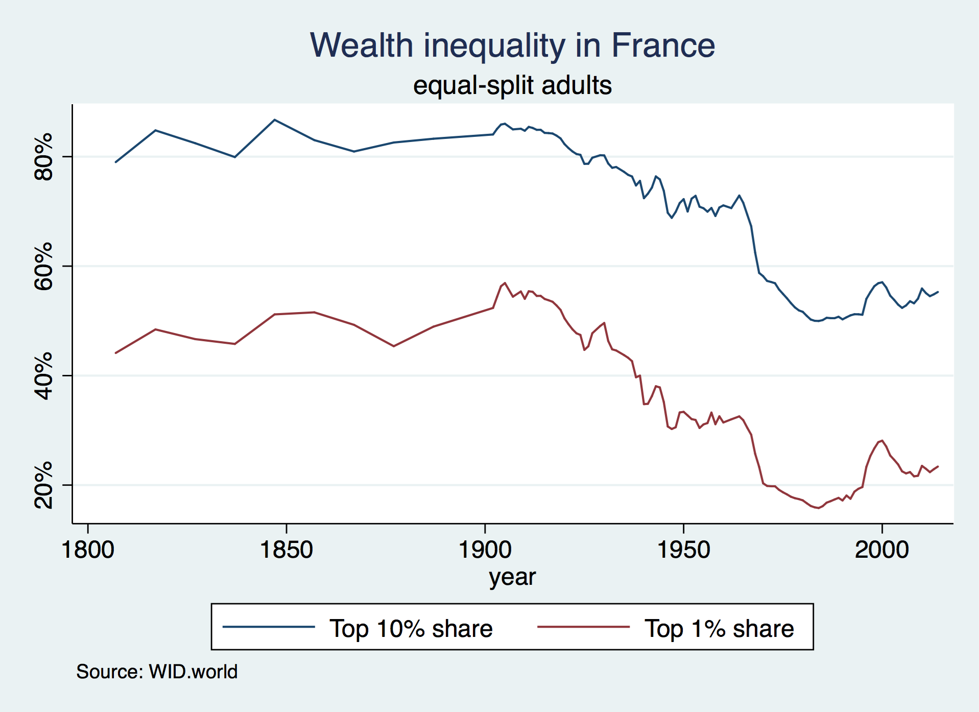

Plot the evolution of the pre-tax national income of the bottom 50% of the population in China, France and the United States since 1978 (in log scale):

// Download and store the 2017 USD PPP exchange rate
wid, indicators(xlcusp) areas(FR US CN) year(2017) clear
rename value ppp
tempfile ppp
save "`ppp'"

wid, indicators(aptinc) areas(FR US CN) perc(p0p50) year(1978/2017) ages(992) pop(j) clear
merge n:1 country using "`ppp'", nogenerate

// Convert to 2017 USD PPP (thousands)
replace value = value/ppp/1000

// Reshape and plot
keep country year value
reshape wide value, i(year) j(country) string
label variable valueFR "France"
label variable valueUS "United States"
label variable valueCN "China"

graph twoway line value* year, yscale(log) ylabel(1 2 5 10 20) ///
	ytitle("2017 PPP USD (000's)") ///
	title("Average pre-tax national income of the bottom 50%") subtitle("equal-split adults") ///
	note("Source: WID.world") legend(rows(1))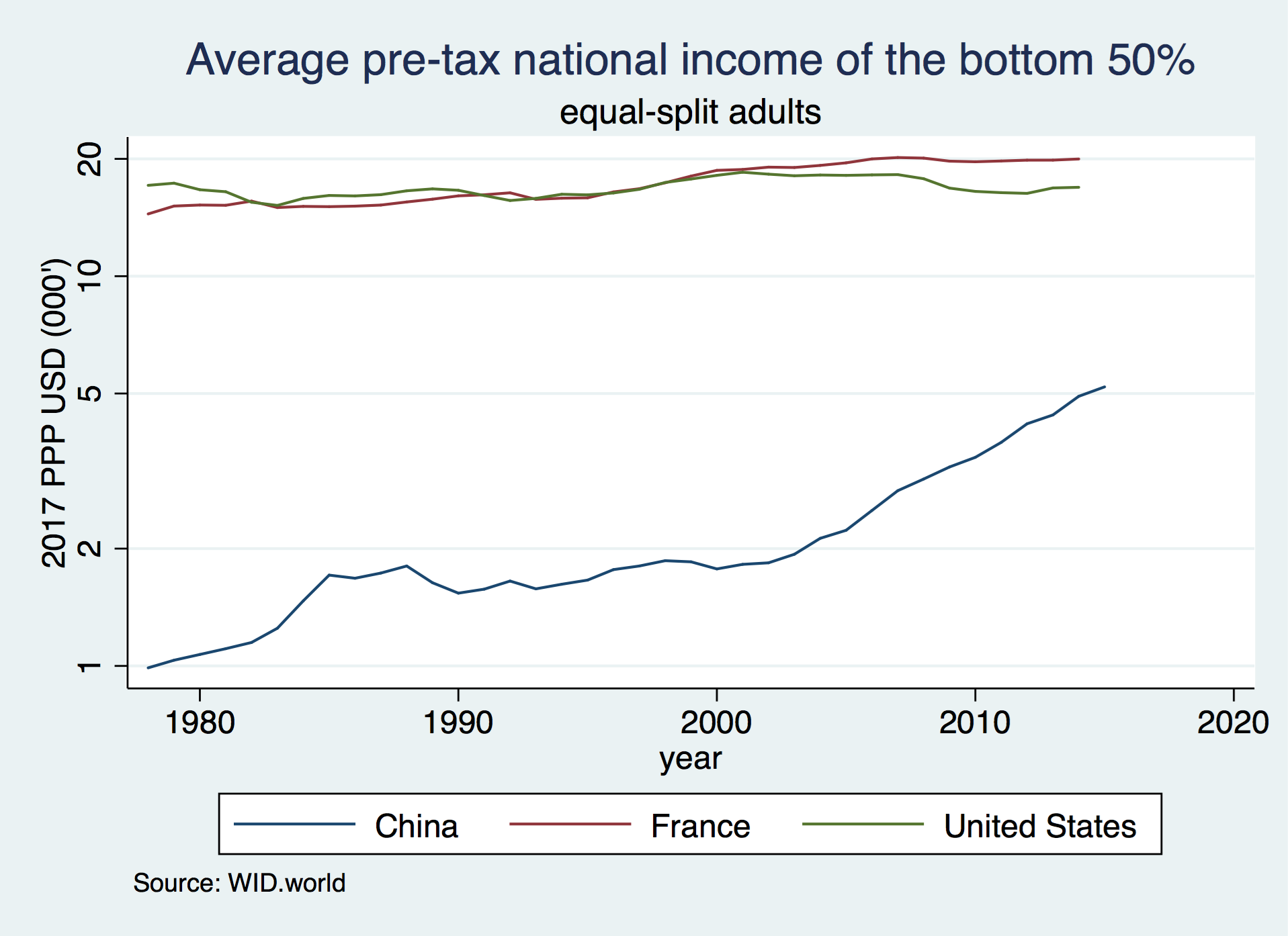

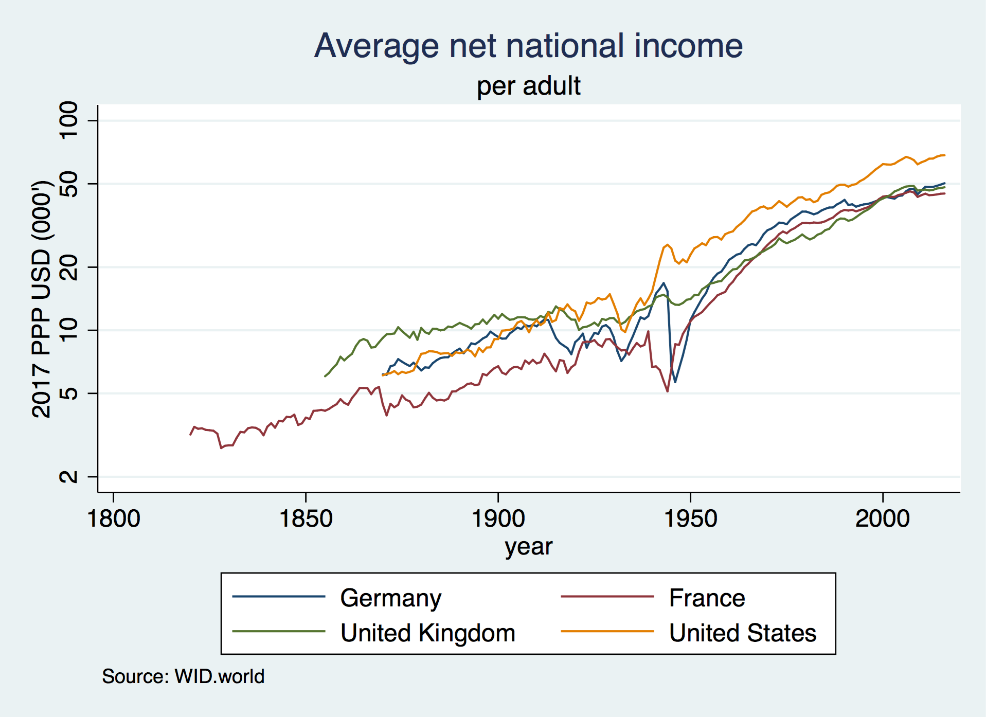
Plot the long-run evolution of average net national income per adult in France, Germany, the United Kingdom and the United States (in log scale):

// Download and store the 2017 USD PPP exchange rate
wid, indicators(xlcusp) areas(FR US DE GB) year(2017) clear
rename value ppp
tempfile ppp
save "`ppp'"

// Download net national income in constant 2017 local currency
wid, indicators(anninc) areas(FR US DE GB) age(992) clear
merge n:1 country using "`ppp'", nogenerate

// Convert to 2017 USD PPP (thousands)
replace value = value/ppp/1000

// Reshape and plot
keep country year value
reshape wide value, i(year) j(country) string
label variable valueFR "France"
label variable valueUS "United States"
label variable valueDE "Germany"
label variable valueGB "United Kingdom"

graph twoway line value* year, yscale(log) ///
	ytitle("2017 PPP USD (000's)") ylabel(2 5 10 20 50 100) ///
	title("Average net national income") subtitle("per adult") ///
	note("Source: WID.world")