Solves the Tower of Hanoi puzzle by reinforcement learning.
In a Python environment with Numpy and Pandas installed, run the script hanoi.py to produce the three plots shown in the Results section. The script can easily be adapted to play the game with a different number of disks N, for example.
Reinforcement learning has recently received renewed interest with the beating of a professional human Go player by Google Deepmind's AlphaGo. Here, a simpler puzzle is solved: the Tower of Hanoi game. The implementation follows the Q-learning algorithm as originally proposed by Watkins & Dayan [1].
The Tower of Hanoi game consists of three pegs and a number of disks of different sizes which can slide onto the pegs. The puzzle starts with all disks stacked on the first peg in ascending order, with the largest at the bottom and the smallest on top. The objective of the game is to move all the disks to the third peg. The only legal moves are those which take the top-most disk from one peg to another, with the restriction that a disk may never be placed upon a smaller disk. Figure 1 shows the optimal solution for 4 disks.

Figure 1. An animated solution of the Tower of Hanoi puzzle for 4 disks. (Source: Wikipedia).
Following Anderson [2], we represent the state of the game by tuples, where the i th element denotes which peg the i th disk is on. The disks are labeled in order of increasing size. Thus, the initial state is (111), and the desired final state is (333) (Figure 2).

Figure 2. Initial and goal states of the Tower of Hanoi puzzle with 3 disks. (From [2]).
The states of the puzzle and the transitions between them corresponding to legal moves form the puzzle's state transition graph, which is shown in Figure 3.
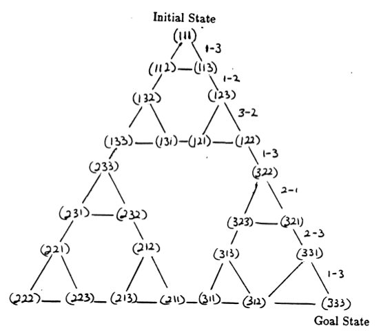
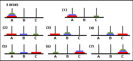
Figure 3. State transition graph for the three-disk Tower of Hanoi puzzle (above) and the corresponding optimal 7-move solution (below), which follows the path of the right hand side of the graph. (From [2] and Mathforum.org).
The minimum number of moves required to solve a Tower of Hanoi puzzle is 2N - 1, where N is the number of disks. Thus for N = 3, the puzzle can be solved in 7 moves, as shown in Figure 3. In the following section, we outline how this is achieved by Q-learning.
R and 'action value' matrix Q for 2 disksThe first step in the program is to generate a reward matrix R which captures the rules of the game and gives a reward for winning it. For simplicity, the reward matrix is shown for N = 2 disks in Figure 4.

Figure 4. Reward matrix R for a Tower of Hanoi puzzle with N = 2 disks. The (i,j)th element represents the reward for moving from state i to j. The states are labeled by tuples as in Figures 2 and 3, with the difference that pegs are indexed 'pythonically' from 0 to 2 rather than from 1 to 3. Moves which lead to the goal state (2,2) are assigned a reward of 100, illegal moves of , and all other moves of 0.
The reward matrix R describes only immediate rewards: a reward of 100 can only be achieved from the penultimate states (0,2) and (1,2). In the other states, each of the 2 or 3 possible moves has an equal reward of 0, and there is no apparent reason to choose one over the other.
Ultimately, we seek to assign a 'value' to each possible move in each state, so that by maximizing over these values we can define a policy leading to the optimal solution. The matrix of 'values' for each action in each state is called Q and can be recursively solved for, or 'learned', in a stochastic manner as described by Watkins & Dayan [1]. The result for 2 disks is shown in Figure 5.

Figure 5. 'Action value' matrix Q for the Tower of Hanoi game with 2 disks, learned with a discount factor of = 0.8, learning factor = 1.0, and 1000 training episodes.
The values of the matrix Q are essentially weights which can be assigned to vertices of the state transition graph in Figure 3, which guide the agent from the initial state to the goal state in the shortest possible way. In this example, by starting at state (0,0) and sucessively choosing the move with the highest value of Q, the reader can convince himself that the Q matrix leads the agent through the sequence of states (0,0) - (1,0) - (1,2) - (2,2), which corresponds to the 3-move optimum solution of the 2-disk Tower of Hanoi game (Figure 6).

Figure 6. Solution of the Tower of Hanoi game with 2 disks. The consecutive states are represented by (0,0), (1,0), (1,2), and (2,2), respectively. (Source: mathforum.org).
In this example where the matrix Q has converged to its optimal value, it defines a stationary policy: each row contains one action with a unique maximum value. During the learning process, however, different actions might have the same value of Q. (In particular, this is the case at the onset of training when Q is initialized to a matrix of zeros). In the simulations presented in the following section, such situations are dealt with by the following stochastic policy: in cases where the maximum Q-value is shared among several actions, choose one of these actions at random.
The performance of the Q-learning algorithm can be measured by counting the number of moves it takes (on average) to solve the Tower of Hanoi puzzle. This number decreases with the number of training episodes until it eventually reaches the optimum value 2N - 1, where N is the number of disks, as illustrated in Figure 7 for N = 2, 3, and 4.
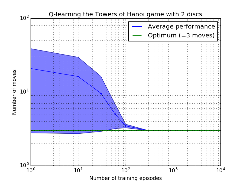
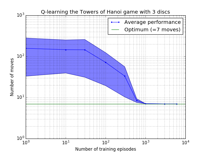
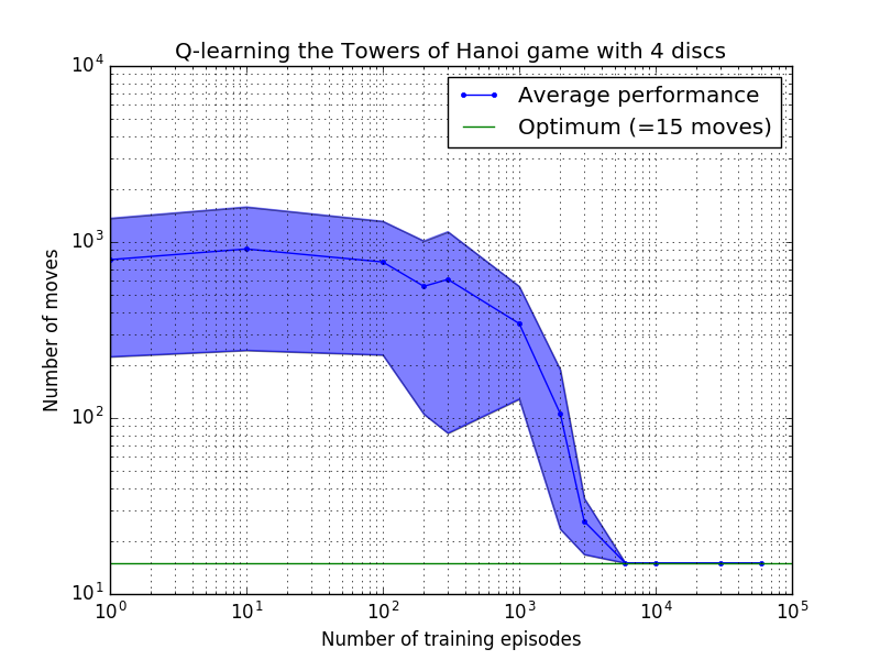
Figure 7. Performance of the Q-learning algorithm for the Tower of Hanoi game with, from top to bottom, 2, 3, and 4 disks. In all cases learning was performed with a discount factor of = 0.8 and a learning factor of = 1.0. The solid blue curve represents the average performance over 100 epochs of training and playing the game 100 times for each resulting stochastic policy. The upper and lower bounds of the shaded blue area are offset from the mean by the estimated standard deviation. (For N = 3 and N = 4, the number of training episodes and times to play were reduced to 10 and 10, respectively, due to computational constraints).
An interesting feature of the learning characteristics in Figure 7 is that in all cases, learning is slow initially, and the agent hardly does better than the 'zero training' policy of choosing moves at random. At some point the learning reaches an 'inflection point' and then converges to the optimal number of moves at an accelerated pace (although this is somewhat exaggerated by the logarithmic scale).
A Python script successfully solves the Tower of Hanoi puzzle optimally for any number of disks by Q-learning. The script can be easily adapted to other problems with a different reward matrix R.
The number of training episodes required to converge to an optimal solution increases greatly with the number of disks N: for N=2 disks it takes ~300 episodes, whereas for N=4 it takes ~6,000. A possible improvement of the learning algorithm would be to allow it to automatically look for recursive solutions, as done by Hengst [3].
[ 1 ] Watkins & Dayan, Q-learning, Machine Learning, 8, 279-292 (1992). (PDF).
[ 2 ] Anderson, Learning and Problem Solving with Multilayer Connectionist Systems, Ph.D. thesis (1986). (PDF).
[ 3 ] Hengst, Discovering Hierarchy in Reinforcement Learning with HEXQ, Proceedings on the Nineteenth International Conference on Machine Learning (2002). (PDF).