vit pytorch
1.9.1

Implementación de Vision Transformer, una forma sencilla de lograr SOTA en la clasificación de visión con un solo codificador de transformador, en Pytorch. El significado se explica con más detalle en el vídeo de Yannic Kilcher. Realmente no hay mucho que codificar aquí, pero también podemos presentarlo para todos para acelerar la revolución de la atención.
Para una implementación de Pytorch con modelos previamente entrenados, consulte el repositorio de Ross Wightman aquí.
El repositorio oficial de Jax está aquí.
¡Aquí también existe una traducción de tensorflow2, creada por el científico investigador Junho Kim!
¡Traducción de lino de Enrico Shippole!
$ pip install vit-pytorch import torch
from vit_pytorch import ViT
v = ViT (
image_size = 256 ,
patch_size = 32 ,
num_classes = 1000 ,
dim = 1024 ,
depth = 6 ,
heads = 16 ,
mlp_dim = 2048 ,
dropout = 0.1 ,
emb_dropout = 0.1
)
img = torch . randn ( 1 , 3 , 256 , 256 )
preds = v ( img ) # (1, 1000) image_size : int.patch_size : int.image_size debe ser divisible por patch_size .n = (image_size // patch_size) ** 2 y n debe ser mayor que 16 .num_classes : int.dim : int.nn.Linear(..., dim) .depth : int.heads : int.mlp_dim :int.channels : int, predeterminado 3 .dropout : flota entre [0, 1] , valor predeterminado 0. .emb_dropout : flota entre [0, 1] , predeterminado 0 .pool : cadena, ya sea agrupación de tokens cls o agrupación mean Una actualización de algunos de los mismos autores del artículo original propone simplificaciones para ViT que le permiten entrenar más rápido y mejor.
Entre estas simplificaciones se incluyen la incrustación posicional sinusoidal 2D, la agrupación promedio global (sin token CLS), sin abandono, tamaños de lote de 1024 en lugar de 4096 y el uso de aumentos RandAugment y MixUp. También muestran que un lineal simple al final no es significativamente peor que la cabeza MLP original.
Puede usarlo importando SimpleViT como se muestra a continuación
 import torch
from vit_pytorch import SimpleViT

v = SimpleViT (
    image_size = 256 ,
    patch_size = 32 ,
    num_classes = 1000 ,
    dim = 1024 ,
    depth = 6 ,
    heads = 16 ,
    mlp_dim = 2048
)

img = torch . randn ( 1 , 3 , 256 , 256 )

preds = v ( img ) # (1, 1000) 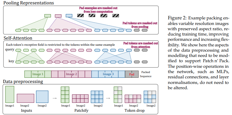
Este artículo propone aprovechar la flexibilidad de la atención y el enmascaramiento de secuencias de longitud variable para entrenar imágenes de resolución múltiple, empaquetadas en un solo lote. Demuestran una capacitación mucho más rápida y una precisión mejorada, con el único costo de una complejidad adicional en la arquitectura y la carga de datos. Utilizan codificaciones posicionales 2D factorizadas, caída de tokens y normalización de claves de consulta.
Puedes usarlo de la siguiente manera
 import torch
from vit_pytorch . na_vit import NaViT

v = NaViT (
    image_size = 256 ,
    patch_size = 32 ,
    num_classes = 1000 ,
    dim = 1024 ,
    depth = 6 ,
    heads = 16 ,
    mlp_dim = 2048 ,
    dropout = 0.1 ,
    emb_dropout = 0.1 ,
    token_dropout_prob = 0.1  # token dropout of 10% (keep 90% of tokens)
)

# 5 images of different resolutions - List[List[Tensor]]

# for now, you'll have to correctly place images in same batch element as to not exceed maximum allowed sequence length for self-attention w/ masking

images = [
    [ torch . randn ( 3 , 256 , 256 ), torch . randn ( 3 , 128 , 128 )],
    [ torch . randn ( 3 , 128 , 256 ), torch . randn ( 3 , 256 , 128 )],
    [ torch . randn ( 3 , 64 , 256 )]
]

preds = v ( images ) # (5, 1000) - 5, because 5 images of different resolution above
O si prefiere que el marco agrupe automáticamente las imágenes en secuencias de longitud variable que no superen una determinada longitud máxima.
 images = [
    torch . randn ( 3 , 256 , 256 ),
    torch . randn ( 3 , 128 , 128 ),
    torch . randn ( 3 , 128 , 256 ),
    torch . randn ( 3 , 256 , 128 ),
    torch . randn ( 3 , 64 , 256 )
]

preds = v (
    images ,
    group_images = True ,
    group_max_seq_len = 64
) # (5, 1000)
Finalmente, si desea utilizar una versión de NaViT usando tensores anidados (que omitirán gran parte del enmascaramiento y el relleno), asegúrese de estar en la versión 2.5 e importe de la siguiente manera
 import torch
from vit_pytorch . na_vit_nested_tensor import NaViT

v = NaViT (
    image_size = 256 ,
    patch_size = 32 ,
    num_classes = 1000 ,
    dim = 1024 ,
    depth = 6 ,
    heads = 16 ,
    mlp_dim = 2048 ,
    dropout = 0. ,
    emb_dropout = 0. ,
    token_dropout_prob = 0.1
)

# 5 images of different resolutions - List[Tensor]

images = [
    torch . randn ( 3 , 256 , 256 ), torch . randn ( 3 , 128 , 128 ),
    torch . randn ( 3 , 128 , 256 ), torch . randn ( 3 , 256 , 128 ),
    torch . randn ( 3 , 64 , 256 )
]

preds = v ( images )

assert preds . shape == ( 5 , 1000 )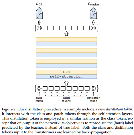
Un artículo reciente ha demostrado que el uso de un token de destilación para destilar conocimientos de redes convolucionales a un transformador de visión puede generar transformadores de visión pequeños y eficientes. Este repositorio ofrece los medios para realizar la destilación fácilmente.
ex. destilando de Resnet50 (o cualquier maestro) a un transformador de visión
 import torch
from torchvision . models import resnet50

from vit_pytorch . distill import DistillableViT , DistillWrapper

teacher = resnet50 ( pretrained = True )

v = DistillableViT (
    image_size = 256 ,
    patch_size = 32 ,
    num_classes = 1000 ,
    dim = 1024 ,
    depth = 6 ,
    heads = 8 ,
    mlp_dim = 2048 ,
    dropout = 0.1 ,
    emb_dropout = 0.1
)

distiller = DistillWrapper (
    student = v ,
    teacher = teacher ,
    temperature = 3 ,           # temperature of distillation
    alpha = 0.5 ,               # trade between main loss and distillation loss
    hard = False               # whether to use soft or hard distillation
)

img = torch . randn ( 2 , 3 , 256 , 256 )
labels = torch . randint ( 0 , 1000 , ( 2 ,))

loss = distiller ( img , labels )
loss . backward ()

# after lots of training above ...

pred = v ( img ) # (2, 1000)
La clase DistillableViT es idéntica a ViT excepto en cómo se maneja el pase hacia adelante, por lo que debería poder cargar los parámetros nuevamente en ViT después de haber completado el entrenamiento de destilación.
También puede utilizar el práctico método .to_vit en la instancia DistillableViT para recuperar una instancia ViT .
 v = v . to_vit ()
type ( v ) # <class 'vit_pytorch.vit_pytorch.ViT'> Este artículo señala que ViT tiene dificultades para atender a mayores profundidades (más allá de las 12 capas) y sugiere mezclar la atención de cada cabeza post-softmax como una solución, denominada Re-atención. Los resultados coinciden con el artículo de Talking Heads de PNL.
Puedes usarlo de la siguiente manera
 import torch
from vit_pytorch . deepvit import DeepViT

v = DeepViT (
    image_size = 256 ,
    patch_size = 32 ,
    num_classes = 1000 ,
    dim = 1024 ,
    depth = 6 ,
    heads = 16 ,
    mlp_dim = 2048 ,
    dropout = 0.1 ,
    emb_dropout = 0.1
)

img = torch . randn ( 1 , 3 , 256 , 256 )

preds = v ( img ) # (1, 1000) Este artículo también señala la dificultad para entrenar transformadores de visión a mayores profundidades y propone dos soluciones. Primero, propone realizar una multiplicación por canal de la salida del bloque residual. En segundo lugar, propone que los parches se atiendan entre sí y solo permita que el token CLS se ocupe de los parches en las últimas capas.
También agregan Talking Heads y notan mejoras.
Puede utilizar este esquema de la siguiente manera
 import torch
from vit_pytorch . cait import CaiT

v = CaiT (
    image_size = 256 ,
    patch_size = 32 ,
    num_classes = 1000 ,
    dim = 1024 ,
    depth = 12 ,             # depth of transformer for patch to patch attention only
    cls_depth = 2 ,          # depth of cross attention of CLS tokens to patch
    heads = 16 ,
    mlp_dim = 2048 ,
    dropout = 0.1 ,
    emb_dropout = 0.1 ,
    layer_dropout = 0.05    # randomly dropout 5% of the layers
)

img = torch . randn ( 1 , 3 , 256 , 256 )

preds = v ( img ) # (1, 1000) 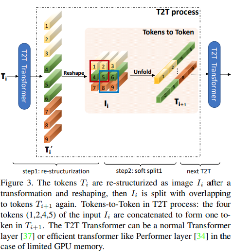
Este artículo propone que las primeras dos capas deben reducir la resolución de la secuencia de imágenes desplegándolas, lo que lleva a la superposición de datos de imagen en cada token, como se muestra en la figura anterior. Puede utilizar esta variante del ViT de la siguiente manera.
 import torch
from vit_pytorch . t2t import T2TViT

v = T2TViT (
    dim = 512 ,
    image_size = 224 ,
    depth = 5 ,
    heads = 8 ,
    mlp_dim = 512 ,
    num_classes = 1000 ,
    t2t_layers = (( 7 , 4 ), ( 3 , 2 ), ( 3 , 2 )) # tuples of the kernel size and stride of each consecutive layers of the initial token to token module
)

img = torch . randn ( 1 , 3 , 224 , 224 )

preds = v ( img ) # (1, 1000)
CCT propone transformadores compactos mediante el uso de convoluciones en lugar de parchear y realizar agrupaciones de secuencias. Esto permite que CCT tenga una alta precisión y una baja cantidad de parámetros.
Puedes usar esto con dos métodos.
 import torch
from vit_pytorch . cct import CCT

cct = CCT (
    img_size = ( 224 , 448 ),
    embedding_dim = 384 ,
    n_conv_layers = 2 ,
    kernel_size = 7 ,
    stride = 2 ,
    padding = 3 ,
    pooling_kernel_size = 3 ,
    pooling_stride = 2 ,
    pooling_padding = 1 ,
    num_layers = 14 ,
    num_heads = 6 ,
    mlp_ratio = 3. ,
    num_classes = 1000 ,
    positional_embedding = 'learnable' , # ['sine', 'learnable', 'none']
)

img = torch . randn ( 1 , 3 , 224 , 448 )
pred = cct ( img ) # (1, 1000)
Alternativamente, puede utilizar uno de varios modelos predefinidos [2,4,6,7,8,14,16] que predefinen el número de capas, el número de cabezales de atención, la relación mlp y la dimensión de incrustación.
 import torch
from vit_pytorch . cct import cct_14

cct = cct_14 (
    img_size = 224 ,
    n_conv_layers = 1 ,
    kernel_size = 7 ,
    stride = 2 ,
    padding = 3 ,
    pooling_kernel_size = 3 ,
    pooling_stride = 2 ,
    pooling_padding = 1 ,
    num_classes = 1000 ,
    positional_embedding = 'learnable' , # ['sine', 'learnable', 'none']
)
El repositorio oficial incluye enlaces a puntos de control de modelos previamente entrenados.
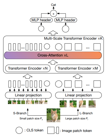
Este artículo propone tener dos transformadores de visión procesando la imagen a diferentes escalas, atendiendo uno de vez en cuando. Muestran mejoras además del transformador de visión base.
 import torch
from vit_pytorch . cross_vit import CrossViT

v = CrossViT (
    image_size = 256 ,
    num_classes = 1000 ,
    depth = 4 ,               # number of multi-scale encoding blocks
    sm_dim = 192 ,            # high res dimension
    sm_patch_size = 16 ,      # high res patch size (should be smaller than lg_patch_size)
    sm_enc_depth = 2 ,        # high res depth
    sm_enc_heads = 8 ,        # high res heads
    sm_enc_mlp_dim = 2048 ,   # high res feedforward dimension
    lg_dim = 384 ,            # low res dimension
    lg_patch_size = 64 ,      # low res patch size
    lg_enc_depth = 3 ,        # low res depth
    lg_enc_heads = 8 ,        # low res heads
    lg_enc_mlp_dim = 2048 ,   # low res feedforward dimensions
    cross_attn_depth = 2 ,    # cross attention rounds
    cross_attn_heads = 8 ,    # cross attention heads
    dropout = 0.1 ,
    emb_dropout = 0.1
)

img = torch . randn ( 1 , 3 , 256 , 256 )

pred = v ( img ) # (1, 1000) 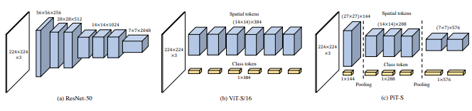
Este artículo propone reducir la muestra de los tokens mediante un procedimiento de agrupación utilizando convoluciones en profundidad.
 import torch
from vit_pytorch . pit import PiT

v = PiT (
    image_size = 224 ,
    patch_size = 14 ,
    dim = 256 ,
    num_classes = 1000 ,
    depth = ( 3 , 3 , 3 ),     # list of depths, indicating the number of rounds of each stage before a downsample
    heads = 16 ,
    mlp_dim = 2048 ,
    dropout = 0.1 ,
    emb_dropout = 0.1
)

# forward pass now returns predictions and the attention maps

img = torch . randn ( 1 , 3 , 224 , 224 )

preds = v ( img ) # (1, 1000) 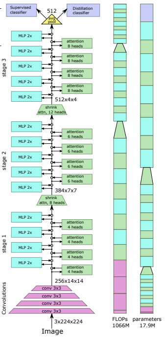
Este artículo propone una serie de cambios, que incluyen (1) incrustación convolucional en lugar de proyección por parches (2) reducción de resolución en etapas (3) no linealidad adicional en la atención (4) sesgos posicionales relativos 2d en lugar de sesgos posicionales absolutos iniciales (5 ) norma de lote en lugar de norma de capa.
Repositorio oficial
 import torch
from vit_pytorch . levit import LeViT

levit = LeViT (
    image_size = 224 ,
    num_classes = 1000 ,
    stages = 3 ,             # number of stages
    dim = ( 256 , 384 , 512 ),  # dimensions at each stage
    depth = 4 ,              # transformer of depth 4 at each stage
    heads = ( 4 , 6 , 8 ),      # heads at each stage
    mlp_mult = 2 ,
    dropout = 0.1
)

img = torch . randn ( 1 , 3 , 224 , 224 )

levit ( img ) # (1, 1000) 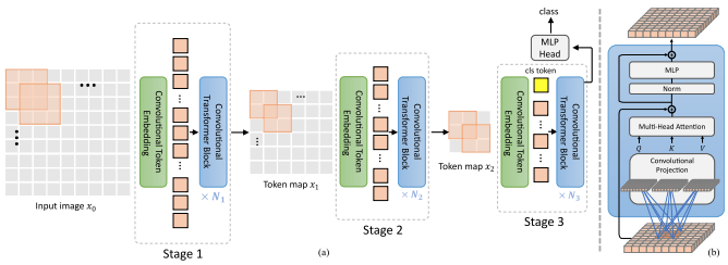
Este artículo propone mezclar convoluciones y atención. Específicamente, las convoluciones se utilizan para incrustar y reducir la resolución de la imagen/mapa de características en tres etapas. La convolución en profundidad también se utiliza para proyectar las consultas, claves y valores a los que prestar atención.
 import torch
from vit_pytorch . cvt import CvT

v = CvT (
    num_classes = 1000 ,
    s1_emb_dim = 64 ,        # stage 1 - dimension
    s1_emb_kernel = 7 ,      # stage 1 - conv kernel
    s1_emb_stride = 4 ,      # stage 1 - conv stride
    s1_proj_kernel = 3 ,     # stage 1 - attention ds-conv kernel size
    s1_kv_proj_stride = 2 ,  # stage 1 - attention key / value projection stride
    s1_heads = 1 ,           # stage 1 - heads
    s1_depth = 1 ,           # stage 1 - depth
    s1_mlp_mult = 4 ,        # stage 1 - feedforward expansion factor
    s2_emb_dim = 192 ,       # stage 2 - (same as above)
    s2_emb_kernel = 3 ,
    s2_emb_stride = 2 ,
    s2_proj_kernel = 3 ,
    s2_kv_proj_stride = 2 ,
    s2_heads = 3 ,
    s2_depth = 2 ,
    s2_mlp_mult = 4 ,
    s3_emb_dim = 384 ,       # stage 3 - (same as above)
    s3_emb_kernel = 3 ,
    s3_emb_stride = 2 ,
    s3_proj_kernel = 3 ,
    s3_kv_proj_stride = 2 ,
    s3_heads = 4 ,
    s3_depth = 10 ,
    s3_mlp_mult = 4 ,
    dropout = 0.
)

img = torch . randn ( 1 , 3 , 224 , 224 )

pred = v ( img ) # (1, 1000) 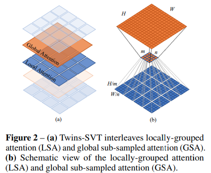
Este artículo propone combinar la atención local y global, junto con el generador de codificación de posición (propuesto en CPVT) y la agrupación promedio global, para lograr los mismos resultados que Swin, sin la complejidad adicional de ventanas desplazadas, tokens CLS ni incrustaciones posicionales.
 import torch
from vit_pytorch . twins_svt import TwinsSVT

model = TwinsSVT (
    num_classes = 1000 ,       # number of output classes
    s1_emb_dim = 64 ,          # stage 1 - patch embedding projected dimension
    s1_patch_size = 4 ,        # stage 1 - patch size for patch embedding
    s1_local_patch_size = 7 ,  # stage 1 - patch size for local attention
    s1_global_k = 7 ,          # stage 1 - global attention key / value reduction factor, defaults to 7 as specified in paper
    s1_depth = 1 ,             # stage 1 - number of transformer blocks (local attn -> ff -> global attn -> ff)
    s2_emb_dim = 128 ,         # stage 2 (same as above)
    s2_patch_size = 2 ,
    s2_local_patch_size = 7 ,
    s2_global_k = 7 ,
    s2_depth = 1 ,
    s3_emb_dim = 256 ,         # stage 3 (same as above)
    s3_patch_size = 2 ,
    s3_local_patch_size = 7 ,
    s3_global_k = 7 ,
    s3_depth = 5 ,
    s4_emb_dim = 512 ,         # stage 4 (same as above)
    s4_patch_size = 2 ,
    s4_local_patch_size = 7 ,
    s4_global_k = 7 ,
    s4_depth = 4 ,
    peg_kernel_size = 3 ,      # positional encoding generator kernel size
    dropout = 0.              # dropout
)

img = torch . randn ( 1 , 3 , 224 , 224 )

pred = model ( img ) # (1, 1000) 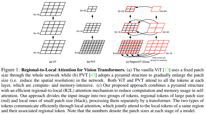
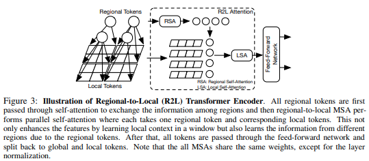
Este artículo propone dividir el mapa de características en regiones locales, mediante las cuales los tokens locales se atienden entre sí. Cada región local tiene su propio token regional que luego atiende a todos sus tokens locales, así como a otros tokens regionales.
Puedes usarlo de la siguiente manera
 import torch
from vit_pytorch . regionvit import RegionViT

model = RegionViT (
    dim = ( 64 , 128 , 256 , 512 ),      # tuple of size 4, indicating dimension at each stage
    depth = ( 2 , 2 , 8 , 2 ),           # depth of the region to local transformer at each stage
    window_size = 7 ,                # window size, which should be either 7 or 14
    num_classes = 1000 ,             # number of output classes
    tokenize_local_3_conv = False ,  # whether to use a 3 layer convolution to encode the local tokens from the image. the paper uses this for the smaller models, but uses only 1 conv (set to False) for the larger models
    use_peg = False ,                # whether to use positional generating module. they used this for object detection for a boost in performance
)

img = torch . randn ( 1 , 3 , 224 , 224 )

pred = model ( img ) # (1, 1000) 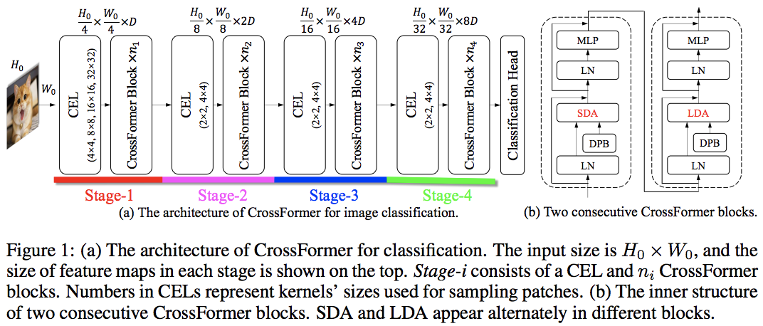
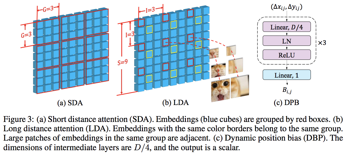
Este artículo supera a PVT y Swin al utilizar atención local y global alternada. La atención global se realiza a través de la dimensión de la ventana para reducir la complejidad, de forma muy similar al esquema utilizado para la atención axial.
También tienen una capa de incrustación de escala cruzada, que demostraron ser una capa genérica que puede mejorar todos los transformadores de visión. También se formuló un sesgo posicional relativo dinámico para permitir que la red se generalice a imágenes de mayor resolución.
 import torch
from vit_pytorch . crossformer import CrossFormer

model = CrossFormer (
    num_classes = 1000 ,                # number of output classes
    dim = ( 64 , 128 , 256 , 512 ),         # dimension at each stage
    depth = ( 2 , 2 , 8 , 2 ),              # depth of transformer at each stage
    global_window_size = ( 8 , 4 , 2 , 1 ), # global window sizes at each stage
    local_window_size = 7 ,             # local window size (can be customized for each stage, but in paper, held constant at 7 for all stages)
)

img = torch . randn ( 1 , 3 , 224 , 224 )

pred = model ( img ) # (1, 1000) 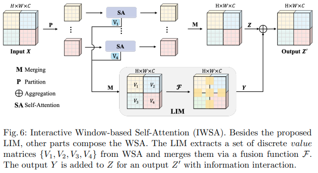
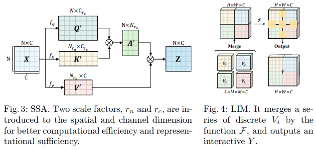
Este artículo de Bytedance AI propone los módulos Scalable Self Attention (SSA) y Interactive Windowed Self Attention (IWSA). El SSA alivia el cálculo necesario en etapas anteriores al reducir el mapa de características clave/valor en algún factor ( reduction_factor ), mientras modula la dimensión de las consultas y claves ( ssa_dim_key ). IWSA realiza autoatención dentro de las ventanas locales, de manera similar a otros papeles transformadores de visión. Sin embargo, agregan un residuo de los valores, pasados a través de una convolución de tamaño de núcleo 3, a la que denominaron Módulo interactivo local (LIM).
En este documento afirman que este esquema supera a Swin Transformer y también demuestra un rendimiento competitivo frente a Crossformer.
Puede usarlo de la siguiente manera (por ejemplo, ScalableViT-S)
 import torch
from vit_pytorch . scalable_vit import ScalableViT

model = ScalableViT (
    num_classes = 1000 ,
    dim = 64 ,                               # starting model dimension. at every stage, dimension is doubled
    heads = ( 2 , 4 , 8 , 16 ),                  # number of attention heads at each stage
    depth = ( 2 , 2 , 20 , 2 ),                  # number of transformer blocks at each stage
    ssa_dim_key = ( 40 , 40 , 40 , 32 ),         # the dimension of the attention keys (and queries) for SSA. in the paper, they represented this as a scale factor on the base dimension per key (ssa_dim_key / dim_key)
    reduction_factor = ( 8 , 4 , 2 , 1 ),        # downsampling of the key / values in SSA. in the paper, this was represented as (reduction_factor ** -2)
    window_size = ( 64 , 32 , None , None ),     # window size of the IWSA at each stage. None means no windowing needed
    dropout = 0.1 ,                          # attention and feedforward dropout
)

img = torch . randn ( 1 , 3 , 256 , 256 )

preds = model ( img ) # (1, 1000) 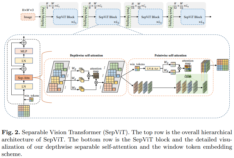
Otro artículo de Bytedance AI, propone una capa de autoatención en profundidad y punto que parece inspirada en gran medida por la convolución separable en profundidad de mobilenet. El aspecto más interesante es la reutilización del mapa de características de la etapa de autoatención profunda como valores para la autoatención puntual, como se muestra en el diagrama anterior.
He decidido incluir solo la versión de SepViT con esta capa de autoatención específica, ya que las capas de atención agrupadas no son destacables ni novedosas, y los autores no tenían claro cómo trataron los tokens de ventana para la capa de autoatención grupal. Además, parece que solo con la capa DSSA , pudieron vencer a Swin.
ex. SepViT-Lite
 import torch
from vit_pytorch . sep_vit import SepViT

v = SepViT (
    num_classes = 1000 ,
    dim = 32 ,               # dimensions of first stage, which doubles every stage (32, 64, 128, 256) for SepViT-Lite
    dim_head = 32 ,          # attention head dimension
    heads = ( 1 , 2 , 4 , 8 ),   # number of heads per stage
    depth = ( 1 , 2 , 6 , 2 ),   # number of transformer blocks per stage
    window_size = 7 ,        # window size of DSS Attention block
    dropout = 0.1           # dropout
)

img = torch . randn ( 1 , 3 , 224 , 224 )

preds = v ( img ) # (1, 1000) 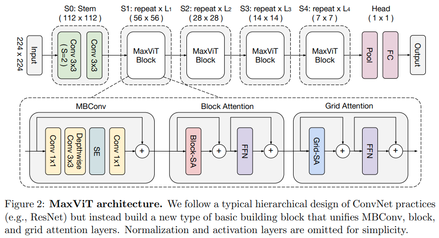
Este artículo propone una red híbrida convolucional/atención, que utiliza MBConv desde el lado convolucional y luego atención dispersa axial de bloque/cuadrícula.
También afirman que este transformador de visión específico es bueno para los modelos generativos (GAN).
ex. MaxViT-S
 import torch
from vit_pytorch . max_vit import MaxViT

v = MaxViT (
    num_classes = 1000 ,
    dim_conv_stem = 64 ,               # dimension of the convolutional stem, would default to dimension of first layer if not specified
    dim = 96 ,                         # dimension of first layer, doubles every layer
    dim_head = 32 ,                    # dimension of attention heads, kept at 32 in paper
    depth = ( 2 , 2 , 5 , 2 ),             # number of MaxViT blocks per stage, which consists of MBConv, block-like attention, grid-like attention
    window_size = 7 ,                  # window size for block and grids
    mbconv_expansion_rate = 4 ,        # expansion rate of MBConv
    mbconv_shrinkage_rate = 0.25 ,     # shrinkage rate of squeeze-excitation in MBConv
    dropout = 0.1                     # dropout
)

img = torch . randn ( 2 , 3 , 224 , 224 )

preds = v ( img ) # (2, 1000) 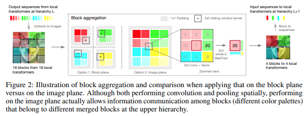
Este artículo decidió procesar la imagen en etapas jerárquicas, con atención solo dentro de los tokens de los bloques locales, que se agregan a medida que se asciende en la jerarquía. La agregación se realiza en el plano de la imagen y contiene una convolución y un grupo máximo posterior para permitirle pasar información a través del límite.
Puedes usarlo con el siguiente código (ej. NesT-T)
 import torch
from vit_pytorch . nest import NesT

nest = NesT (
    image_size = 224 ,
    patch_size = 4 ,
    dim = 96 ,
    heads = 3 ,
    num_hierarchies = 3 ,        # number of hierarchies
    block_repeats = ( 2 , 2 , 8 ),  # the number of transformer blocks at each hierarchy, starting from the bottom
    num_classes = 1000
)

img = torch . randn ( 1 , 3 , 224 , 224 )

pred = nest ( img ) # (1, 1000) 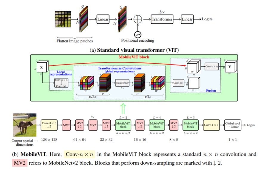
Este artículo presenta MobileViT, un transformador de visión liviano y de uso general para dispositivos móviles. MobileViT presenta una perspectiva diferente para el procesamiento global de información con transformadores.
Puedes usarlo con el siguiente código (ej. mobilevit_xs)
 import torch
from vit_pytorch . mobile_vit import MobileViT

mbvit_xs = MobileViT (
    image_size = ( 256 , 256 ),
    dims = [ 96 , 120 , 144 ],
    channels = [ 16 , 32 , 48 , 48 , 64 , 64 , 80 , 80 , 96 , 96 , 384 ],
    num_classes = 1000
)

img = torch . randn ( 1 , 3 , 256 , 256 )

pred = mbvit_xs ( img ) # (1, 1000) 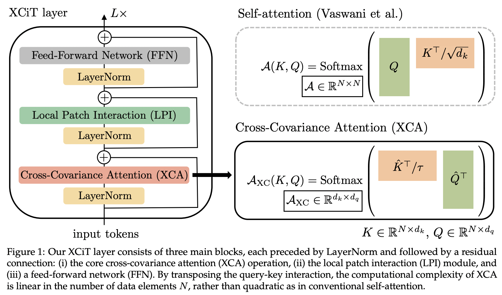
Este artículo presenta la atención de covarianza cruzada (abreviada XCA). Se puede pensar que se presta atención a través de la dimensión de características en lugar de la espacial (otra perspectiva sería una convolución dinámica 1x1, cuyo núcleo sería un mapa de atención definido por correlaciones espaciales).
Técnicamente, esto equivale simplemente a transponer los valores clave y de consulta antes de ejecutar la atención de similitud del coseno con la temperatura aprendida.
 import torch
from vit_pytorch . xcit import XCiT

v = XCiT (
    image_size = 256 ,
    patch_size = 32 ,
    num_classes = 1000 ,
    dim = 1024 ,
    depth = 12 ,                     # depth of xcit transformer
    cls_depth = 2 ,                  # depth of cross attention of CLS tokens to patch, attention pool at end
    heads = 16 ,
    mlp_dim = 2048 ,
    dropout = 0.1 ,
    emb_dropout = 0.1 ,
    layer_dropout = 0.05 ,           # randomly dropout 5% of the layers
    local_patch_kernel_size = 3     # kernel size of the local patch interaction module (depthwise convs)
)

img = torch . randn ( 1 , 3 , 256 , 256 )

preds = v ( img ) # (1, 1000) 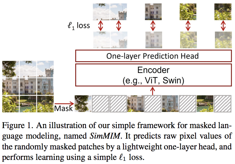
Este artículo propone un esquema simple de modelado de imágenes enmascaradas (SimMIM), utilizando solo una proyección lineal de los tokens enmascarados en el espacio de píxeles seguida de una pérdida L1 con los valores de píxeles de los parches enmascarados. Los resultados son competitivos con otros enfoques más complicados.
Puedes usar esto de la siguiente manera
 import torch
from vit_pytorch import ViT
from vit_pytorch . simmim import SimMIM

v = ViT (
    image_size = 256 ,
    patch_size = 32 ,
    num_classes = 1000 ,
    dim = 1024 ,
    depth = 6 ,
    heads = 8 ,
    mlp_dim = 2048
)

mim = SimMIM (
    encoder = v ,
    masking_ratio = 0.5  # they found 50% to yield the best results
)

images = torch . randn ( 8 , 3 , 256 , 256 )

loss = mim ( images )
loss . backward ()

# that's all!
# do the above in a for loop many times with a lot of images and your vision transformer will learn

torch . save ( v . state_dict (), './trained-vit.pt' )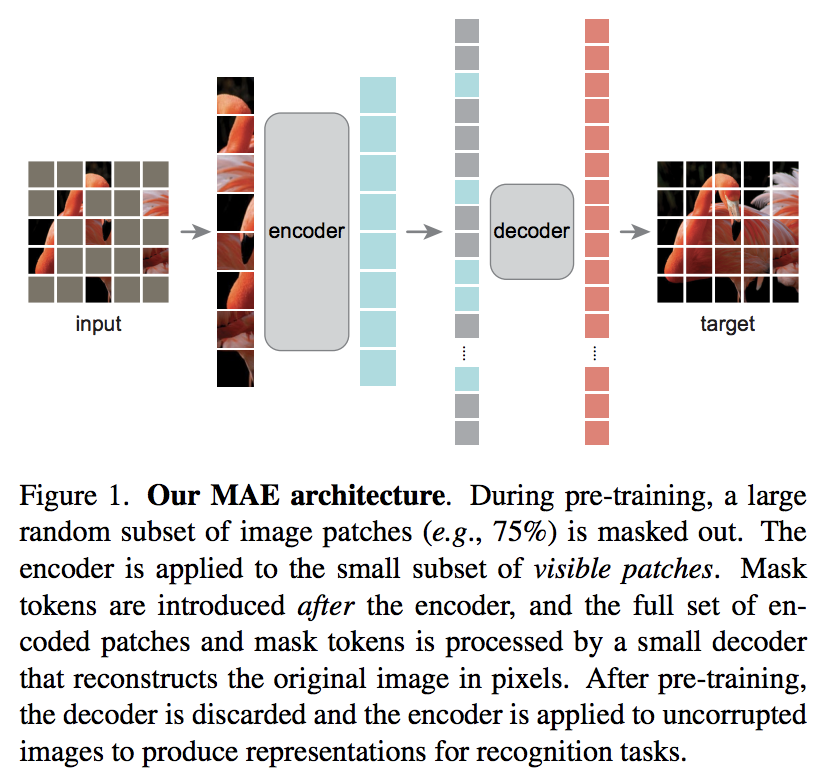
Un nuevo artículo de Kaiming He propone un esquema de codificador automático simple en el que el transformador de visión atiende a un conjunto de parches desenmascarados y un decodificador más pequeño intenta reconstruir los valores de píxeles enmascarados.
Revisión rápida del artículo de DeepReader
Coffeebreak AI con Letitia
Puedes usarlo con el siguiente código.
 import torch
from vit_pytorch import ViT , MAE

v = ViT (
    image_size = 256 ,
    patch_size = 32 ,
    num_classes = 1000 ,
    dim = 1024 ,
    depth = 6 ,
    heads = 8 ,
    mlp_dim = 2048
)

mae = MAE (
    encoder = v ,
    masking_ratio = 0.75 ,   # the paper recommended 75% masked patches
    decoder_dim = 512 ,      # paper showed good results with just 512
    decoder_depth = 6       # anywhere from 1 to 8
)

images = torch . randn ( 8 , 3 , 256 , 256 )

loss = mae ( images )
loss . backward ()

# that's all!
# do the above in a for loop many times with a lot of images and your vision transformer will learn

# save your improved vision transformer
torch . save ( v . state_dict (), './trained-vit.pt' )Gracias a Zach, puedes entrenar usando la tarea de predicción de parches enmascarados original presentada en el artículo, con el siguiente código.
 import torch
from vit_pytorch import ViT
from vit_pytorch . mpp import MPP

model = ViT (
    image_size = 256 ,
    patch_size = 32 ,
    num_classes = 1000 ,
    dim = 1024 ,
    depth = 6 ,
    heads = 8 ,
    mlp_dim = 2048 ,
    dropout = 0.1 ,
    emb_dropout = 0.1
)

mpp_trainer = MPP (
    transformer = model ,
    patch_size = 32 ,
    dim = 1024 ,
    mask_prob = 0.15 ,          # probability of using token in masked prediction task
    random_patch_prob = 0.30 ,  # probability of randomly replacing a token being used for mpp
    replace_prob = 0.50 ,       # probability of replacing a token being used for mpp with the mask token
)

opt = torch . optim . Adam ( mpp_trainer . parameters (), lr = 3e-4 )

def sample_unlabelled_images ():
    return torch . FloatTensor ( 20 , 3 , 256 , 256 ). uniform_ ( 0. , 1. )

for _ in range ( 100 ):
    images = sample_unlabelled_images ()
    loss = mpp_trainer ( images )
    opt . zero_grad ()
    loss . backward ()
    opt . step ()

# save your improved network
torch . save ( model . state_dict (), './pretrained-net.pt' )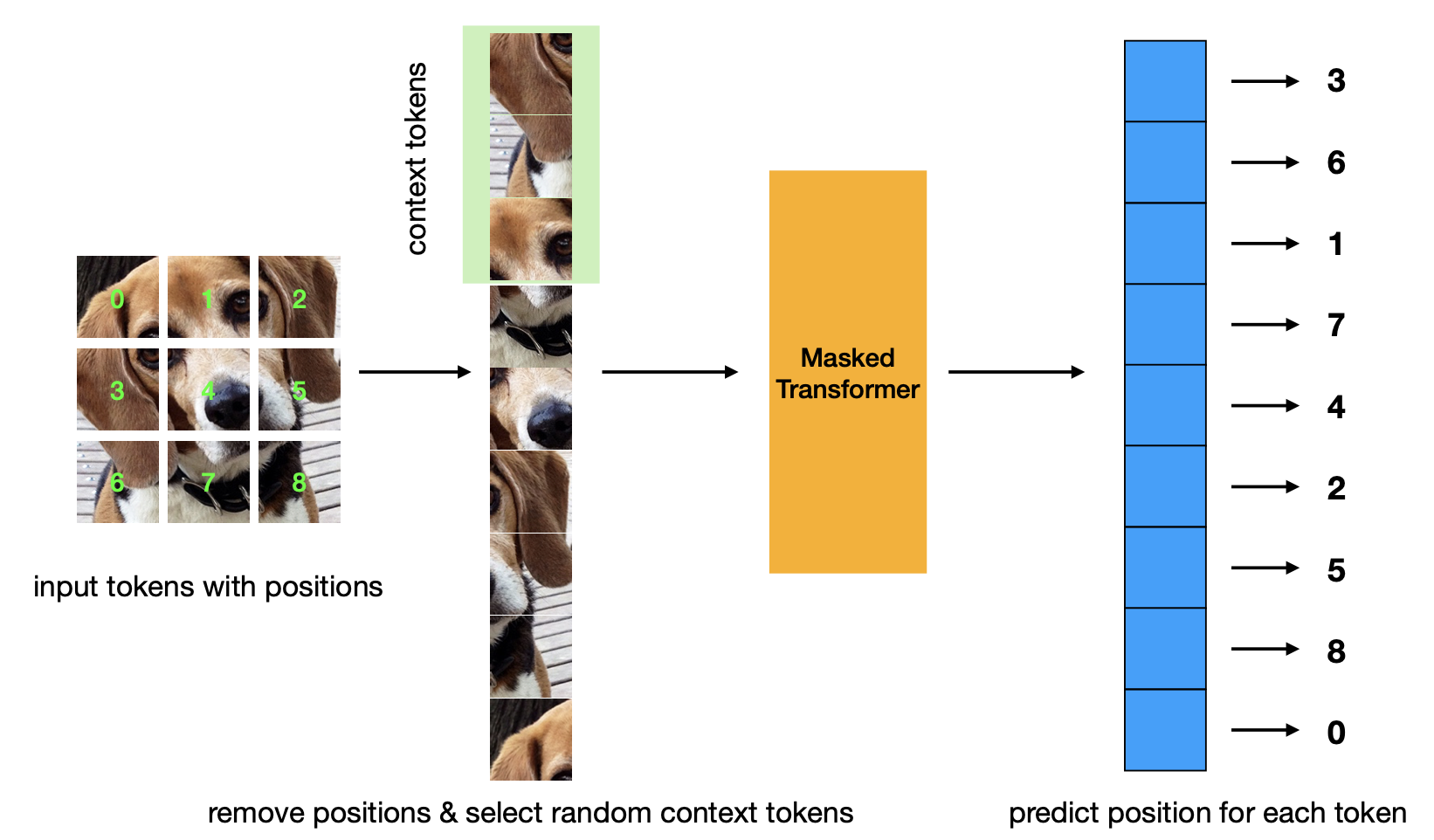
Nuevo artículo que presenta criterios de preentrenamiento de predicción de posiciones enmascaradas. Esta estrategia es más eficiente que la estrategia Masked Autoencoder y tiene un rendimiento comparable.
 import torch
from vit_pytorch . mp3 import ViT , MP3

v = ViT (
    num_classes = 1000 ,
    image_size = 256 ,
    patch_size = 8 ,
    dim = 1024 ,
    depth = 6 ,
    heads = 8 ,
    mlp_dim = 2048 ,
    dropout = 0.1 ,
)

mp3 = MP3 (
    vit = v ,
    masking_ratio = 0.75
)

images = torch . randn ( 8 , 3 , 256 , 256 )

loss = mp3 ( images )
loss . backward ()

# that's all!
# do the above in a for loop many times with a lot of images and your vision transformer will learn

# save your improved vision transformer
torch . save ( v . state_dict (), './trained-vit.pt' )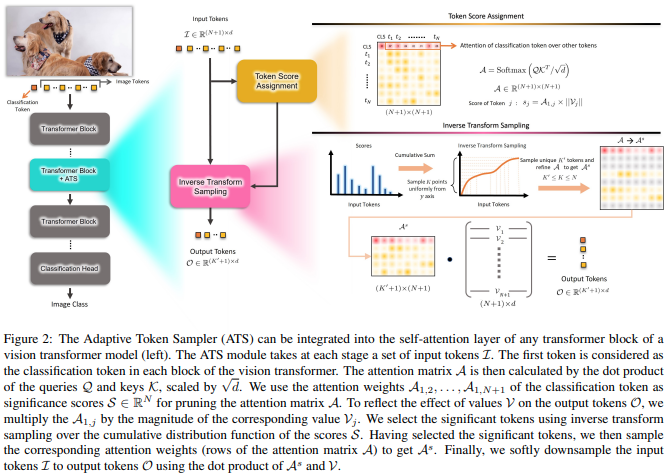
Este artículo propone utilizar las puntuaciones de atención de CLS, ponderadas nuevamente por las normas de los jefes de valor, como medio para descartar tokens sin importancia en diferentes capas.
 import torch
from vit_pytorch . ats_vit import ViT

v = ViT (
    image_size = 256 ,
    patch_size = 16 ,
    num_classes = 1000 ,
    dim = 1024 ,
    depth = 6 ,
    max_tokens_per_depth = ( 256 , 128 , 64 , 32 , 16 , 8 ), # a tuple that denotes the maximum number of tokens that any given layer should have. if the layer has greater than this amount, it will undergo adaptive token sampling
    heads = 16 ,
    mlp_dim = 2048 ,
    dropout = 0.1 ,
    emb_dropout = 0.1
)

img = torch . randn ( 4 , 3 , 256 , 256 )

preds = v ( img ) # (4, 1000)

# you can also get a list of the final sampled patch ids
# a value of -1 denotes padding

preds , token_ids = v ( img , return_sampled_token_ids = True ) # (4, 1000), (4, <=8) 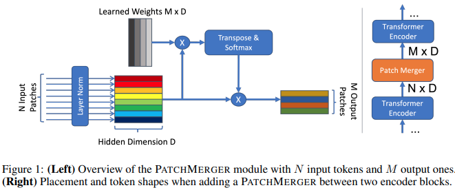
Este artículo propone un módulo simple (Patch Merger) para reducir la cantidad de tokens en cualquier capa de un transformador de visión sin sacrificar el rendimiento.
 import torch
from vit_pytorch . vit_with_patch_merger import ViT

v = ViT (
    image_size = 256 ,
    patch_size = 16 ,
    num_classes = 1000 ,
    dim = 1024 ,
    depth = 12 ,
    heads = 8 ,
    patch_merge_layer = 6 ,        # at which transformer layer to do patch merging
    patch_merge_num_tokens = 8 ,   # the output number of tokens from the patch merge
    mlp_dim = 2048 ,
    dropout = 0.1 ,
    emb_dropout = 0.1
)

img = torch . randn ( 4 , 3 , 256 , 256 )

preds = v ( img ) # (4, 1000)
También se puede utilizar el módulo PatchMerger por sí solo.
 import torch
from vit_pytorch . vit_with_patch_merger import PatchMerger

merger = PatchMerger (
    dim = 1024 ,
    num_tokens_out = 8   # output number of tokens
)

features = torch . randn ( 4 , 256 , 1024 ) # (batch, num tokens, dimension)

out = merger ( features ) # (4, 8, 1024) 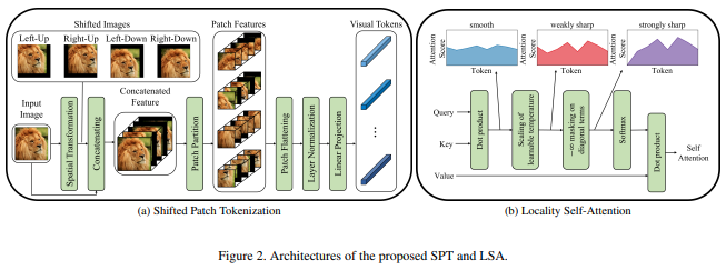
Este artículo propone una nueva función de imagen para parchear que incorpora cambios de la imagen, antes de normalizar y dividir la imagen en parches. Descubrí que el cambio es extremadamente útil en otros trabajos con transformadores, por lo que decidí incluir esto para futuras exploraciones. También incluye el LSA con la temperatura aprendida y el enmascaramiento de la atención del token hacia sí mismo.
Puedes utilizar lo siguiente:
 import torch
from vit_pytorch . vit_for_small_dataset import ViT

v = ViT (
    image_size = 256 ,
    patch_size = 16 ,
    num_classes = 1000 ,
    dim = 1024 ,
    depth = 6 ,
    heads = 16 ,
    mlp_dim = 2048 ,
    dropout = 0.1 ,
    emb_dropout = 0.1
)

img = torch . randn ( 4 , 3 , 256 , 256 )

preds = v ( img ) # (1, 1000)
También puede utilizar el SPT de este documento como módulo independiente.
 import torch
from vit_pytorch . vit_for_small_dataset import SPT

spt = SPT (
    dim = 1024 ,
    patch_size = 16 ,
    channels = 3
)

img = torch . randn ( 4 , 3 , 256 , 256 )

tokens = spt ( img ) # (4, 256, 1024) Por petición popular, comenzaré a extender algunas de las arquitecturas de este repositorio a ViT 3D, para usar con video, imágenes médicas, etc.
Deberá pasar dos hiperparámetros adicionales: (1) el número de frames y (2) el tamaño del parche a lo largo de la dimensión del cuadro frame_patch_size
Para empezar, 3D ViT
 import torch
from vit_pytorch . vit_3d import ViT

v = ViT (
    image_size = 128 ,          # image size
    frames = 16 ,               # number of frames
    image_patch_size = 16 ,     # image patch size
    frame_patch_size = 2 ,      # frame patch size
    num_classes = 1000 ,
    dim = 1024 ,
    depth = 6 ,
    heads = 8 ,
    mlp_dim = 2048 ,
    dropout = 0.1 ,
    emb_dropout = 0.1
)

video = torch . randn ( 4 , 3 , 16 , 128 , 128 ) # (batch, channels, frames, height, width)

preds = v ( video ) # (4, 1000)
ViT simple 3D
 import torch
from vit_pytorch . simple_vit_3d import SimpleViT

v = SimpleViT (
    image_size = 128 ,          # image size
    frames = 16 ,               # number of frames
    image_patch_size = 16 ,     # image patch size
    frame_patch_size = 2 ,      # frame patch size
    num_classes = 1000 ,
    dim = 1024 ,
    depth = 6 ,
    heads = 8 ,
    mlp_dim = 2048
)

video = torch . randn ( 4 , 3 , 16 , 128 , 128 ) # (batch, channels, frames, height, width)

preds = v ( video ) # (4, 1000)
Versión 3D de CCT
 import torch
from vit_pytorch . cct_3d import CCT

cct = CCT (
    img_size = 224 ,
    num_frames = 8 ,
    embedding_dim = 384 ,
    n_conv_layers = 2 ,
    frame_kernel_size = 3 ,
    kernel_size = 7 ,
    stride = 2 ,
    padding = 3 ,
    pooling_kernel_size = 3 ,
    pooling_stride = 2 ,
    pooling_padding = 1 ,
    num_layers = 14 ,
    num_heads = 6 ,
    mlp_ratio = 3. ,
    num_classes = 1000 ,
    positional_embedding = 'learnable'
)

video = torch . randn ( 1 , 3 , 8 , 224 , 224 ) # (batch, channels, frames, height, width)
pred = cct ( video )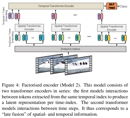
Este artículo ofrece 3 tipos diferentes de arquitecturas para la atención eficiente de videos, siendo el tema principal factorizar la atención a través del espacio y el tiempo. Este repositorio incluye el codificador factorizado y la variante de autoatención factorizada. La variante del codificador factorizado es un transformador espacial seguido de uno temporal. La variante de autoatención factorizada es un transformador espacio-temporal con capas de autoatención espaciales y temporales alternas.
 import torch
from vit_pytorch . vivit import ViT

v = ViT (
    image_size = 128 ,          # image size
    frames = 16 ,               # number of frames
    image_patch_size = 16 ,     # image patch size
    frame_patch_size = 2 ,      # frame patch size
    num_classes = 1000 ,
    dim = 1024 ,
    spatial_depth = 6 ,         # depth of the spatial transformer
    temporal_depth = 6 ,        # depth of the temporal transformer
    heads = 8 ,
    mlp_dim = 2048 ,
    variant = 'factorized_encoder' , # or 'factorized_self_attention'
)

video = torch . randn ( 4 , 3 , 16 , 128 , 128 ) # (batch, channels, frames, height, width)

preds = v ( video ) # (4, 1000) 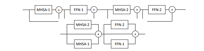
Este artículo propone paralelizar múltiples bloques de atención y retroalimentación por capa (2 bloques), afirmando que es más fácil entrenar sin pérdida de rendimiento.
Puedes probar esta variante de la siguiente manera.
 import torch
from vit_pytorch . parallel_vit import ViT

v = ViT (
    image_size = 256 ,
    patch_size = 16 ,
    num_classes = 1000 ,
    dim = 1024 ,
    depth = 6 ,
    heads = 8 ,
    mlp_dim = 2048 ,
    num_parallel_branches = 2 ,  # in paper, they claimed 2 was optimal
    dropout = 0.1 ,
    emb_dropout = 0.1
)

img = torch . randn ( 4 , 3 , 256 , 256 )

preds = v ( img ) # (4, 1000) 
Este documento muestra que agregar tokens de memoria que se pueden aprender en cada capa de un transformador de visión puede mejorar en gran medida los resultados del ajuste (además del token CLS y el cabezal adaptador específicos de la tarea que se pueden aprender).
Puede utilizar esto con un ViT especialmente modificado de la siguiente manera
 import torch
from vit_pytorch . learnable_memory_vit import ViT , Adapter

# normal base ViT

v = ViT (
    image_size = 256 ,
    patch_size = 16 ,
    num_classes = 1000 ,
    dim = 1024 ,
    depth = 6 ,
    heads = 8 ,
    mlp_dim = 2048 ,
    dropout = 0.1 ,
    emb_dropout = 0.1
)

img = torch . randn ( 4 , 3 , 256 , 256 )
logits = v ( img ) # (4, 1000)

# do your usual training with ViT
# ...


# then, to finetune, just pass the ViT into the Adapter class
# you can do this for multiple Adapters, as shown below

adapter1 = Adapter (
    vit = v ,
    num_classes = 2 ,               # number of output classes for this specific task
    num_memories_per_layer = 5     # number of learnable memories per layer, 10 was sufficient in paper
)

logits1 = adapter1 ( img ) # (4, 2) - predict 2 classes off frozen ViT backbone with learnable memories and task specific head

# yet another task to finetune on, this time with 4 classes

adapter2 = Adapter (
    vit = v ,
    num_classes = 4 ,
    num_memories_per_layer = 10
)

logits2 = adapter2 ( img ) # (4, 4) - predict 4 classes off frozen ViT backbone with learnable memories and task specific head 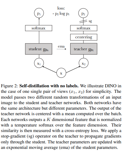
Puede entrenar ViT con la reciente técnica de aprendizaje autosupervisado SOTA, Dino, con el siguiente código.
Vídeo de Yannic Kilcher
 import torch
from vit_pytorch import ViT , Dino

model = ViT (
    image_size = 256 ,
    patch_size = 32 ,
    num_classes = 1000 ,
    dim = 1024 ,
    depth = 6 ,
    heads = 8 ,
    mlp_dim = 2048
)

learner = Dino (
    model ,
    image_size = 256 ,
    hidden_layer = 'to_latent' ,        # hidden layer name or index, from which to extract the embedding
    projection_hidden_size = 256 ,      # projector network hidden dimension
    projection_layers = 4 ,             # number of layers in projection network
    num_classes_K = 65336 ,             # output logits dimensions (referenced as K in paper)
    student_temp = 0.9 ,                # student temperature
    teacher_temp = 0.04 ,               # teacher temperature, needs to be annealed from 0.04 to 0.07 over 30 epochs
    local_upper_crop_scale = 0.4 ,      # upper bound for local crop - 0.4 was recommended in the paper
    global_lower_crop_scale = 0.5 ,     # lower bound for global crop - 0.5 was recommended in the paper
    moving_average_decay = 0.9 ,        # moving average of encoder - paper showed anywhere from 0.9 to 0.999 was ok
    center_moving_average_decay = 0.9 , # moving average of teacher centers - paper showed anywhere from 0.9 to 0.999 was ok
)

opt = torch . optim . Adam ( learner . parameters (), lr = 3e-4 )

def sample_unlabelled_images ():
    return torch . randn ( 20 , 3 , 256 , 256 )

for _ in range ( 100 ):
    images = sample_unlabelled_images ()
    loss = learner ( images )
    opt . zero_grad ()
    loss . backward ()
    opt . step ()
    learner . update_moving_average () # update moving average of teacher encoder and teacher centers

# save your improved network
torch . save ( model . state_dict (), './pretrained-net.pt' )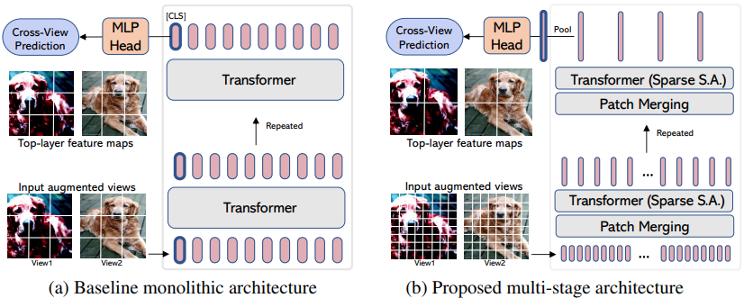
EsViT es una variante de Dino (desde arriba) rediseñada para admitir ViT eficientes con fusión/reducción de resolución de parches teniendo en cuenta una pérdida regional adicional entre las vistas aumentadas. Para citar el resumen, outperforms its supervised counterpart on 17 out of 18 datasets con un rendimiento 3 veces mayor.
Aunque se nombra como si fuera una nueva variante ViT , en realidad es solo una estrategia para entrenar cualquier ViT de múltiples etapas (en el documento, se centraron en Swin). El siguiente ejemplo mostrará cómo usarlo con CvT . Deberá configurar la hidden_layer con el nombre de la capa dentro de su ViT eficiente que genera las representaciones visuales agrupadas no promedio, justo antes de la agrupación global y la proyección a logits.
 import torch
from vit_pytorch . cvt import CvT
from vit_pytorch . es_vit import EsViTTrainer

cvt = CvT (
    num_classes = 1000 ,
    s1_emb_dim = 64 ,
    s1_emb_kernel = 7 ,
    s1_emb_stride = 4 ,
    s1_proj_kernel = 3 ,
    s1_kv_proj_stride = 2 ,
    s1_heads = 1 ,
    s1_depth = 1 ,
    s1_mlp_mult = 4 ,
    s2_emb_dim = 192 ,
    s2_emb_kernel = 3 ,
    s2_emb_stride = 2 ,
    s2_proj_kernel = 3 ,
    s2_kv_proj_stride = 2 ,
    s2_heads = 3 ,
    s2_depth = 2 ,
    s2_mlp_mult = 4 ,
    s3_emb_dim = 384 ,
    s3_emb_kernel = 3 ,
    s3_emb_stride = 2 ,
    s3_proj_kernel = 3 ,
    s3_kv_proj_stride = 2 ,
    s3_heads = 4 ,
    s3_depth = 10 ,
    s3_mlp_mult = 4 ,
    dropout = 0.
)

learner = EsViTTrainer (
    cvt ,
    image_size = 256 ,
    hidden_layer = 'layers' ,           # hidden layer name or index, from which to extract the embedding
    projection_hidden_size = 256 ,      # projector network hidden dimension
    projection_layers = 4 ,             # number of layers in projection network
    num_classes_K = 65336 ,             # output logits dimensions (referenced as K in paper)
    student_temp = 0.9 ,                # student temperature
    teacher_temp = 0.04 ,               # teacher temperature, needs to be annealed from 0.04 to 0.07 over 30 epochs
    local_upper_crop_scale = 0.4 ,      # upper bound for local crop - 0.4 was recommended in the paper
    global_lower_crop_scale = 0.5 ,     # lower bound for global crop - 0.5 was recommended in the paper
    moving_average_decay = 0.9 ,        # moving average of encoder - paper showed anywhere from 0.9 to 0.999 was ok
    center_moving_average_decay = 0.9 , # moving average of teacher centers - paper showed anywhere from 0.9 to 0.999 was ok
)

opt = torch . optim . AdamW ( learner . parameters (), lr = 3e-4 )

def sample_unlabelled_images ():
    return torch . randn ( 8 , 3 , 256 , 256 )

for _ in range ( 1000 ):
    images = sample_unlabelled_images ()
    loss = learner ( images )
    opt . zero_grad ()
    loss . backward ()
    opt . step ()
    learner . update_moving_average () # update moving average of teacher encoder and teacher centers

# save your improved network
torch . save ( cvt . state_dict (), './pretrained-net.pt' )Si desea visualizar los pesos de atención (post-softmax) para su investigación, simplemente siga el procedimiento a continuación
 import torch
from vit_pytorch . vit import ViT

v = ViT (
    image_size = 256 ,
    patch_size = 32 ,
    num_classes = 1000 ,
    dim = 1024 ,
    depth = 6 ,
    heads = 16 ,
    mlp_dim = 2048 ,
    dropout = 0.1 ,
    emb_dropout = 0.1
)

# import Recorder and wrap the ViT

from vit_pytorch . recorder import Recorder
v = Recorder ( v )

# forward pass now returns predictions and the attention maps

img = torch . randn ( 1 , 3 , 256 , 256 )
preds , attns = v ( img )

# there is one extra patch due to the CLS token

attns # (1, 6, 16, 65, 65) - (batch x layers x heads x patch x patch)
para limpiar la clase y los ganchos una vez que haya recopilado suficientes datos
v = v . eject () # wrapper is discarded and original ViT instance is returned De manera similar, puede acceder a las incrustaciones con el contenedor Extractor
 import torch
from vit_pytorch . vit import ViT

v = ViT (
    image_size = 256 ,
    patch_size = 32 ,
    num_classes = 1000 ,
    dim = 1024 ,
    depth = 6 ,
    heads = 16 ,
    mlp_dim = 2048 ,
    dropout = 0.1 ,
    emb_dropout = 0.1
)

# import Recorder and wrap the ViT

from vit_pytorch . extractor import Extractor
v = Extractor ( v )

# forward pass now returns predictions and the attention maps

img = torch . randn ( 1 , 3 , 256 , 256 )
logits , embeddings = v ( img )

# there is one extra token due to the CLS token

embeddings # (1, 65, 1024) - (batch x patches x model dim)
O digamos CrossViT , que tiene un codificador multiescala que genera dos conjuntos de incrustaciones para escalas "grandes" y "pequeñas".
 import torch
from vit_pytorch . cross_vit import CrossViT

v = CrossViT (
    image_size = 256 ,
    num_classes = 1000 ,
    depth = 4 ,
    sm_dim = 192 ,
    sm_patch_size = 16 ,
    sm_enc_depth = 2 ,
    sm_enc_heads = 8 ,
    sm_enc_mlp_dim = 2048 ,
    lg_dim = 384 ,
    lg_patch_size = 64 ,
    lg_enc_depth = 3 ,
    lg_enc_heads = 8 ,
    lg_enc_mlp_dim = 2048 ,
    cross_attn_depth = 2 ,
    cross_attn_heads = 8 ,
    dropout = 0.1 ,
    emb_dropout = 0.1
)

# wrap the CrossViT

from vit_pytorch . extractor import Extractor
v = Extractor ( v , layer_name = 'multi_scale_encoder' ) # take embedding coming from the output of multi-scale-encoder

# forward pass now returns predictions and the attention maps

img = torch . randn ( 1 , 3 , 256 , 256 )
logits , embeddings = v ( img )

# there is one extra token due to the CLS token

embeddings # ((1, 257, 192), (1, 17, 384)) - (batch x patches x dimension) <- large and small scales respectively Es posible que algunos provenientes de la visión por computadora piensen que la atención todavía sufre costos cuadráticos. Afortunadamente, tenemos muchas técnicas nuevas que pueden ayudar. Este repositorio ofrece una manera de conectar su propio transformador de atención dispersa.
Un ejemplo con Nystromformer
$ pip install nystrom-attention import torch
from vit_pytorch . efficient import ViT
from nystrom_attention import Nystromformer
efficient_transformer = Nystromformer (
dim = 512 ,
depth = 12 ,
heads = 8 ,
num_landmarks = 256
)
v = ViT (
dim = 512 ,
image_size = 2048 ,
patch_size = 32 ,
num_classes = 1000 ,
transformer = efficient_transformer
)
img = torch . randn ( 1 , 3 , 2048 , 2048 ) # your high resolution picture
v ( img ) # (1, 1000)Otros marcos de atención escasa que recomendaría encarecidamente son Routing Transformer o Sinkhorn Transformer.
Este artículo utilizó deliberadamente las redes de atención más básicas para hacer una declaración. Si desea utilizar algunas de las últimas mejoras para las redes de atención, utilice el Encoder de este repositorio.
ex.
$ pip install x-transformers import torch
from vit_pytorch . efficient import ViT
from x_transformers import Encoder
v = ViT (
dim = 512 ,
image_size = 224 ,
patch_size = 16 ,
num_classes = 1000 ,
transformer = Encoder (
dim = 512 , # set to be the same as the wrapper
depth = 12 ,
heads = 8 ,
ff_glu = True , # ex. feed forward GLU variant https://arxiv.org/abs/2002.05202
residual_attn = True # ex. residual attention https://arxiv.org/abs/2012.11747
)
)
img = torch . randn ( 1 , 3 , 224 , 224 )
v ( img ) # (1, 1000) Ya puedes pasar imágenes que no sean cuadradas; solo debes asegurarte de que la altura y el ancho sean menores o iguales que image_size y que ambos sean divisibles por patch_size
ex.
 import torch
from vit_pytorch import ViT

v = ViT (
    image_size = 256 ,
    patch_size = 32 ,
    num_classes = 1000 ,
    dim = 1024 ,
    depth = 6 ,
    heads = 16 ,
    mlp_dim = 2048 ,
    dropout = 0.1 ,
    emb_dropout = 0.1
)

img = torch . randn ( 1 , 3 , 256 , 128 ) # <-- not a square

preds = v ( img ) # (1, 1000) import torch
from vit_pytorch import ViT
v = ViT (
num_classes = 1000 ,
image_size = ( 256 , 128 ), # image size is a tuple of (height, width)
patch_size = ( 32 , 16 ), # patch size is a tuple of (height, width)
dim = 1024 ,
depth = 6 ,
heads = 16 ,
mlp_dim = 2048 ,
dropout = 0.1 ,
emb_dropout = 0.1
)
img = torch . randn ( 1 , 3 , 256 , 128 )
preds = v ( img )¿Viene de la visión por computadora y es nuevo en los transformadores? Aquí hay algunos recursos que aceleraron enormemente mi aprendizaje.
Transformador ilustrado - Jay Alammar
Transformadores desde cero - Peter Bloem
El transformador anotado - PNL de Harvard
 @article { hassani2021escaping ,
    title   = { Escaping the Big Data Paradigm with Compact Transformers } ,
    author  = { Ali Hassani and Steven Walton and Nikhil Shah and Abulikemu Abuduweili and Jiachen Li and Humphrey Shi } ,
    year    = 2021 ,
    url     = { https://arxiv.org/abs/2104.05704 } ,
    eprint  = { 2104.05704 } ,
    archiveprefix = { arXiv } ,
    primaryclass = { cs.CV }
}
@misc { dosovitskiy2020image ,
title = { An Image is Worth 16x16 Words: Transformers for Image Recognition at Scale } ,
author = { Alexey Dosovitskiy and Lucas Beyer and Alexander Kolesnikov and Dirk Weissenborn and Xiaohua Zhai and Thomas Unterthiner and Mostafa Dehghani and Matthias Minderer and Georg Heigold and Sylvain Gelly and Jakob Uszkoreit and Neil Houlsby } ,
year = { 2020 } ,
eprint = { 2010.11929 } ,
archivePrefix = { arXiv } ,
primaryClass = { cs.CV }
} @misc { touvron2020training ,
title = { Training data-efficient image transformers & distillation through attention } ,
author = { Hugo Touvron and Matthieu Cord and Matthijs Douze and Francisco Massa and Alexandre Sablayrolles and Hervé Jégou } ,
year = { 2020 } ,
eprint = { 2012.12877 } ,
archivePrefix = { arXiv } ,
primaryClass = { cs.CV }
} @misc { yuan2021tokenstotoken ,
title = { Tokens-to-Token ViT: Training Vision Transformers from Scratch on ImageNet } ,
author = { Li Yuan and Yunpeng Chen and Tao Wang and Weihao Yu and Yujun Shi and Francis EH Tay and Jiashi Feng and Shuicheng Yan } ,
year = { 2021 } ,
eprint = { 2101.11986 } ,
archivePrefix = { arXiv } ,
primaryClass = { cs.CV }
} @misc { zhou2021deepvit ,
title = { DeepViT: Towards Deeper Vision Transformer } ,
author = { Daquan Zhou and Bingyi Kang and Xiaojie Jin and Linjie Yang and Xiaochen Lian and Qibin Hou and Jiashi Feng } ,
year = { 2021 } ,
eprint = { 2103.11886 } ,
archivePrefix = { arXiv } ,
primaryClass = { cs.CV }
} @misc { touvron2021going ,
title = { Going deeper with Image Transformers } ,
author = { Hugo Touvron and Matthieu Cord and Alexandre Sablayrolles and Gabriel Synnaeve and Hervé Jégou } ,
year = { 2021 } ,
eprint = { 2103.17239 } ,
archivePrefix = { arXiv } ,
primaryClass = { cs.CV }
} @misc { chen2021crossvit ,
title = { CrossViT: Cross-Attention Multi-Scale Vision Transformer for Image Classification } ,
author = { Chun-Fu Chen and Quanfu Fan and Rameswar Panda } ,
year = { 2021 } ,
eprint = { 2103.14899 } ,
archivePrefix = { arXiv } ,
primaryClass = { cs.CV }
} @misc { wu2021cvt ,
title = { CvT: Introducing Convolutions to Vision Transformers } ,
author = { Haiping Wu and Bin Xiao and Noel Codella and Mengchen Liu and Xiyang Dai and Lu Yuan and Lei Zhang } ,
year = { 2021 } ,
eprint = { 2103.15808 } ,
archivePrefix = { arXiv } ,
primaryClass = { cs.CV }
} @misc { heo2021rethinking ,
title = { Rethinking Spatial Dimensions of Vision Transformers } ,
author = { Byeongho Heo and Sangdoo Yun and Dongyoon Han and Sanghyuk Chun and Junsuk Choe and Seong Joon Oh } ,
year = { 2021 } ,
eprint = { 2103.16302 } ,
archivePrefix = { arXiv } ,
primaryClass = { cs.CV }
} @misc { graham2021levit ,
title = { LeViT: a Vision Transformer in ConvNet's Clothing for Faster Inference } ,
author = { Ben Graham and Alaaeldin El-Nouby and Hugo Touvron and Pierre Stock and Armand Joulin and Hervé Jégou and Matthijs Douze } ,
year = { 2021 } ,
eprint = { 2104.01136 } ,
archivePrefix = { arXiv } ,
primaryClass = { cs.CV }
} @misc { li2021localvit ,
title = { LocalViT: Bringing Locality to Vision Transformers } ,
author = { Yawei Li and Kai Zhang and Jiezhang Cao and Radu Timofte and Luc Van Gool } ,
year = { 2021 } ,
eprint = { 2104.05707 } ,
archivePrefix = { arXiv } ,
primaryClass = { cs.CV }
} @misc { chu2021twins ,
title = { Twins: Revisiting Spatial Attention Design in Vision Transformers } ,
author = { Xiangxiang Chu and Zhi Tian and Yuqing Wang and Bo Zhang and Haibing Ren and Xiaolin Wei and Huaxia Xia and Chunhua Shen } ,
year = { 2021 } ,
eprint = { 2104.13840 } ,
archivePrefix = { arXiv } ,
primaryClass = { cs.CV }
} @misc { su2021roformer ,
title = { RoFormer: Enhanced Transformer with Rotary Position Embedding } ,
author = { Jianlin Su and Yu Lu and Shengfeng Pan and Bo Wen and Yunfeng Liu } ,
year = { 2021 } ,
eprint = { 2104.09864 } ,
archivePrefix = { arXiv } ,
primaryClass = { cs.CL }
} @misc { zhang2021aggregating ,
title = { Aggregating Nested Transformers } ,
author = { Zizhao Zhang and Han Zhang and Long Zhao and Ting Chen and Tomas Pfister } ,
year = { 2021 } ,
eprint = { 2105.12723 } ,
archivePrefix = { arXiv } ,
primaryClass = { cs.CV }
} @misc { chen2021regionvit ,
title = { RegionViT: Regional-to-Local Attention for Vision Transformers } ,
author = { Chun-Fu Chen and Rameswar Panda and Quanfu Fan } ,
year = { 2021 } ,
eprint = { 2106.02689 } ,
archivePrefix = { arXiv } ,
primaryClass = { cs.CV }
} @misc { wang2021crossformer ,
title = { CrossFormer: A Versatile Vision Transformer Hinging on Cross-scale Attention } ,
author = { Wenxiao Wang and Lu Yao and Long Chen and Binbin Lin and Deng Cai and Xiaofei He and Wei Liu } ,
year = { 2021 } ,
eprint = { 2108.00154 } ,
archivePrefix = { arXiv } ,
primaryClass = { cs.CV }
} @misc { caron2021emerging ,
title = { Emerging Properties in Self-Supervised Vision Transformers } ,
author = { Mathilde Caron and Hugo Touvron and Ishan Misra and Hervé Jégou and Julien Mairal and Piotr Bojanowski and Armand Joulin } ,
year = { 2021 } ,
eprint = { 2104.14294 } ,
archivePrefix = { arXiv } ,
primaryClass = { cs.CV }
} @misc { he2021masked ,
title = { Masked Autoencoders Are Scalable Vision Learners } ,
author = { Kaiming He and Xinlei Chen and Saining Xie and Yanghao Li and Piotr Dollár and Ross Girshick } ,
year = { 2021 } ,
eprint = { 2111.06377 } ,
archivePrefix = { arXiv } ,
primaryClass = { cs.CV }
} @misc { xie2021simmim ,
title = { SimMIM: A Simple Framework for Masked Image Modeling } ,
author = { Zhenda Xie and Zheng Zhang and Yue Cao and Yutong Lin and Jianmin Bao and Zhuliang Yao and Qi Dai and Han Hu } ,
year = { 2021 } ,
eprint = { 2111.09886 } ,
archivePrefix = { arXiv } ,
primaryClass = { cs.CV }
} @misc { fayyaz2021ats ,
title = { ATS: Adaptive Token Sampling For Efficient Vision Transformers } ,
author = { Mohsen Fayyaz and Soroush Abbasi Kouhpayegani and Farnoush Rezaei Jafari and Eric Sommerlade and Hamid Reza Vaezi Joze and Hamed Pirsiavash and Juergen Gall } ,
year = { 2021 } ,
eprint = { 2111.15667 } ,
archivePrefix = { arXiv } ,
primaryClass = { cs.CV }
} @misc { mehta2021mobilevit ,
title = { MobileViT: Light-weight, General-purpose, and Mobile-friendly Vision Transformer } ,
author = { Sachin Mehta and Mohammad Rastegari } ,
year = { 2021 } ,
eprint = { 2110.02178 } ,
archivePrefix = { arXiv } ,
primaryClass = { cs.CV }
} @misc { lee2021vision ,
title = { Vision Transformer for Small-Size Datasets } ,
author = { Seung Hoon Lee and Seunghyun Lee and Byung Cheol Song } ,
year = { 2021 } ,
eprint = { 2112.13492 } ,
archivePrefix = { arXiv } ,
primaryClass = { cs.CV }
} @misc { renggli2022learning ,
title = { Learning to Merge Tokens in Vision Transformers } ,
author = { Cedric Renggli and André Susano Pinto and Neil Houlsby and Basil Mustafa and Joan Puigcerver and Carlos Riquelme } ,
year = { 2022 } ,
eprint = { 2202.12015 } ,
archivePrefix = { arXiv } ,
primaryClass = { cs.CV }
} @misc { yang2022scalablevit ,
title = { ScalableViT: Rethinking the Context-oriented Generalization of Vision Transformer } ,
author = { Rui Yang and Hailong Ma and Jie Wu and Yansong Tang and Xuefeng Xiao and Min Zheng and Xiu Li } ,
year = { 2022 } ,
eprint = { 2203.10790 } ,
archivePrefix = { arXiv } ,
primaryClass = { cs.CV }
} @inproceedings { Touvron2022ThreeTE ,
title = { Three things everyone should know about Vision Transformers } ,
author = { Hugo Touvron and Matthieu Cord and Alaaeldin El-Nouby and Jakob Verbeek and Herv'e J'egou } ,
year = { 2022 }
} @inproceedings { Sandler2022FinetuningIT ,
title = { Fine-tuning Image Transformers using Learnable Memory } ,
author = { Mark Sandler and Andrey Zhmoginov and Max Vladymyrov and Andrew Jackson } ,
year = { 2022 }
} @inproceedings { Li2022SepViTSV ,
title = { SepViT: Separable Vision Transformer } ,
author = { Wei Li and Xing Wang and Xin Xia and Jie Wu and Xuefeng Xiao and Minghang Zheng and Shiping Wen } ,
year = { 2022 }
} @inproceedings { Tu2022MaxViTMV ,
title = { MaxViT: Multi-Axis Vision Transformer } ,
author = { Zhengzhong Tu and Hossein Talebi and Han Zhang and Feng Yang and Peyman Milanfar and Alan Conrad Bovik and Yinxiao Li } ,
year = { 2022 }
} @article { Li2021EfficientSV ,
title = { Efficient Self-supervised Vision Transformers for Representation Learning } ,
author = { Chunyuan Li and Jianwei Yang and Pengchuan Zhang and Mei Gao and Bin Xiao and Xiyang Dai and Lu Yuan and Jianfeng Gao } ,
journal = { ArXiv } ,
year = { 2021 } ,
volume = { abs/2106.09785 }
} @misc { Beyer2022BetterPlainViT
title = { Better plain ViT baselines for ImageNet-1k } ,
author = { Beyer, Lucas and Zhai, Xiaohua and Kolesnikov, Alexander } ,
publisher = { arXiv } ,
year = { 2022 }
}
 @article { Arnab2021ViViTAV ,
    title   = { ViViT: A Video Vision Transformer } ,
    author  = { Anurag Arnab and Mostafa Dehghani and Georg Heigold and Chen Sun and Mario Lucic and Cordelia Schmid } ,
    journal = { 2021 IEEE/CVF International Conference on Computer Vision (ICCV) } ,
    year    = { 2021 } ,
    pages   = { 6816-6826 }
}
@article { Liu2022PatchDropoutEV ,
title = { PatchDropout: Economizing Vision Transformers Using Patch Dropout } ,
author = { Yue Liu and Christos Matsoukas and Fredrik Strand and Hossein Azizpour and Kevin Smith } ,
journal = { ArXiv } ,
year = { 2022 } ,
volume = { abs/2208.07220 }
} @misc { https://doi.org/10.48550/arxiv.2302.01327 ,
doi = { 10.48550/ARXIV.2302.01327 } ,
url = { https://arxiv.org/abs/2302.01327 } ,
author = { Kumar, Manoj and Dehghani, Mostafa and Houlsby, Neil } ,
title = { Dual PatchNorm } ,
publisher = { arXiv } ,
year = { 2023 } ,
copyright = { Creative Commons Attribution 4.0 International }
} @inproceedings { Dehghani2023PatchNP ,
title = { Patch n' Pack: NaViT, a Vision Transformer for any Aspect Ratio and Resolution } ,
author = { Mostafa Dehghani and Basil Mustafa and Josip Djolonga and Jonathan Heek and Matthias Minderer and Mathilde Caron and Andreas Steiner and Joan Puigcerver and Robert Geirhos and Ibrahim M. Alabdulmohsin and Avital Oliver and Piotr Padlewski and Alexey A. Gritsenko and Mario Luvci'c and Neil Houlsby } ,
year = { 2023 }
} @misc { vaswani2017attention ,
title = { Attention Is All You Need } ,
author = { Ashish Vaswani and Noam Shazeer and Niki Parmar and Jakob Uszkoreit and Llion Jones and Aidan N. Gomez and Lukasz Kaiser and Illia Polosukhin } ,
year = { 2017 } ,
eprint = { 1706.03762 } ,
archivePrefix = { arXiv } ,
primaryClass = { cs.CL }
} @inproceedings { dao2022flashattention ,
title = { Flash{A}ttention: Fast and Memory-Efficient Exact Attention with {IO}-Awareness } ,
author = { Dao, Tri and Fu, Daniel Y. and Ermon, Stefano and Rudra, Atri and R{'e}, Christopher } ,
booktitle = { Advances in Neural Information Processing Systems } ,
year = { 2022 }
} @inproceedings { Darcet2023VisionTN ,
title = { Vision Transformers Need Registers } ,
author = { Timoth'ee Darcet and Maxime Oquab and Julien Mairal and Piotr Bojanowski } ,
year = { 2023 } ,
url = { https://api.semanticscholar.org/CorpusID:263134283 }
} @inproceedings { ElNouby2021XCiTCI ,
title = { XCiT: Cross-Covariance Image Transformers } ,
author = { Alaaeldin El-Nouby and Hugo Touvron and Mathilde Caron and Piotr Bojanowski and Matthijs Douze and Armand Joulin and Ivan Laptev and Natalia Neverova and Gabriel Synnaeve and Jakob Verbeek and Herv{'e} J{'e}gou } ,
booktitle = { Neural Information Processing Systems } ,
year = { 2021 } ,
url = { https://api.semanticscholar.org/CorpusID:235458262 }
} @inproceedings { Koner2024LookupViTCV ,
title = { LookupViT: Compressing visual information to a limited number of tokens } ,
author = { Rajat Koner and Gagan Jain and Prateek Jain and Volker Tresp and Sujoy Paul } ,
year = { 2024 } ,
url = { https://api.semanticscholar.org/CorpusID:271244592 }
} @article { Bao2022AllAW ,
title = { All are Worth Words: A ViT Backbone for Diffusion Models } ,
author = { Fan Bao and Shen Nie and Kaiwen Xue and Yue Cao and Chongxuan Li and Hang Su and Jun Zhu } ,
journal = { 2023 IEEE/CVF Conference on Computer Vision and Pattern Recognition (CVPR) } ,
year = { 2022 } ,
pages = { 22669-22679 } ,
url = { https://api.semanticscholar.org/CorpusID:253581703 }
} @misc { Rubin2024 ,
author = { Ohad Rubin } ,
url = { https://medium.com/ @ ohadrubin/exploring-weight-decay-in-layer-normalization-challenges-and-a-reparameterization-solution-ad4d12c24950 }
} @inproceedings { Loshchilov2024nGPTNT ,
title = { nGPT: Normalized Transformer with Representation Learning on the Hypersphere } ,
author = { Ilya Loshchilov and Cheng-Ping Hsieh and Simeng Sun and Boris Ginsburg } ,
year = { 2024 } ,
url = { https://api.semanticscholar.org/CorpusID:273026160 }
} @inproceedings { Liu2017DeepHL ,
title = { Deep Hyperspherical Learning } ,
author = { Weiyang Liu and Yanming Zhang and Xingguo Li and Zhen Liu and Bo Dai and Tuo Zhao and Le Song } ,
booktitle = { Neural Information Processing Systems } ,
year = { 2017 } ,
url = { https://api.semanticscholar.org/CorpusID:5104558 }
} @inproceedings { Zhou2024ValueRL ,
title = { Value Residual Learning For Alleviating Attention Concentration In Transformers } ,
author = { Zhanchao Zhou and Tianyi Wu and Zhiyun Jiang and Zhenzhong Lan } ,
year = { 2024 } ,
url = { https://api.semanticscholar.org/CorpusID:273532030 }
} @article { Zhu2024HyperConnections ,
title = { Hyper-Connections } ,
author = { Defa Zhu and Hongzhi Huang and Zihao Huang and Yutao Zeng and Yunyao Mao and Banggu Wu and Qiyang Min and Xun Zhou } ,
journal = { ArXiv } ,
year = { 2024 } ,
volume = { abs/2409.19606 } ,
url = { https://api.semanticscholar.org/CorpusID:272987528 }
}Visualizo un momento en el que seremos para los robots lo que los perros son para los humanos, y estoy apoyando a las máquinas. —Claude Shannon


