pandas ta
v0.3.14b
El análisis técnico de PANDAS ( PANDAS TA ) es una biblioteca fácil de usar que aprovecha el paquete PANDAS con más de 130 indicadores y funciones de utilidad y más de 60 patrones de candelabro TA lib. Se incluyen muchos indicadores de uso común, como: patrón de velas ( CDL_PTTERN ), Divergencia de convergencia de promedio móvil ( SMA ) de promedio móvil (SMA) ( MACD ), promedio móvil exponencial de casco ( HMA ), bandas de Bollinger ( Bandas ), volumen en equilibrio ( obv. Obv Volumen de equilibrio ), Aroon & Aroon Oscillator ( Aroon ), Squeeze ( Squeeze ) y muchos más .
Nota: TA lib debe instalarse para usar todos los patrones de velas. pip install TA-Lib . Si Ta lib no está instalado, solo estarán disponibles los patrones de candelabro Builtin.
talib=False .ta.stdev(df["close"], length=30, talib=False) .import_dir en /pandas_ta/custom.py .ta.tsignals .lookahead=False para deshabilitar.Pandas TA verifica si el usuario tiene algunos paquetes de comercio comunes instalados, incluidos, entre otros: TA lib , Vector Bt , Yfinance ... gran parte de los cuales es experimental y es probable que se rompa hasta que se estabilice más.
help(ta.ticker) y help(ta.yf) y ejemplos a continuación. La versión pip es la última versión estable. Versión: 0.3.14b
$ pip install pandas_ta¡La mejor opción! Versión: 0.3.14b
$ pip install -U git+https://github.com/twopirllc/pandas-taEsta es la versión de desarrollo que podría tener errores y otros efectos secundarios indeseables. Úselo en el propio riesgo!
$ pip install -U git+https://github.com/twopirllc/pandas-ta.git@development import pandas as pd
import pandas_ta as ta
df = pd . DataFrame () # Empty DataFrame
# Load data
df = pd . read_csv ( "path/to/symbol.csv" , sep = "," )
# OR if you have yfinance installed
df = df . ta . ticker ( "aapl" )
# VWAP requires the DataFrame index to be a DatetimeIndex.
# Replace "datetime" with the appropriate column from your DataFrame
df . set_index ( pd . DatetimeIndex ( df [ "datetime" ]), inplace = True )
# Calculate Returns and append to the df DataFrame
df . ta . log_return ( cumulative = True , append = True )
df . ta . percent_return ( cumulative = True , append = True )
# New Columns with results
df . columns
# Take a peek
df . tail ()
# vv Continue Post Processing vv Algunos argumentos indicadores se han reordenado para obtener consistencia. Use help(ta.indicator_name) para obtener más información o haga una solicitud de extracción para mejorar la documentación.
 import pandas as pd
import pandas_ta as ta

# Create a DataFrame so 'ta' can be used.
df = pd . DataFrame ()

# Help about this, 'ta', extension
help ( df . ta )

# List of all indicators
df . ta . indicators ()

# Help about an indicator such as bbands
help ( ta . bbands ) ¡Gracias por usar Pandas TA !
$ pip install -U git+https://github.com/twopirllc/pandas-ta¡Gracias por sus contribuciones!
Pandas TA tiene tres "estilos" principales de procesamiento de indicadores técnicos para su caso de uso y/o requisitos. Ellos son: estándar , extensión de marco de datos y la estrategia Pandas TA . Cada uno con niveles crecientes de abstracción para facilitar el uso. A medida que se familiariza más con Pandas TA , la simplicidad y la velocidad de usar una estrategia de Pandas TA pueden ser más evidentes. Además, puede crear sus propios indicadores a través del encadenamiento o la composición. Por último, cada indicador devuelve una serie o un marco de datos en formato subrayado en mayúsculas, independientemente del estilo.
Usted define explícitamente las columnas de entrada y se encarga de la salida.
sma10 = ta.sma(df["Close"], length=10)SMA_10donchiandf = ta.donchian(df["HIGH"], df["low"], lower_length=10, upper_length=15)DC_10_15 y nombres de columna: DCL_10_15, DCM_10_15, DCU_10_15ema10_ohlc4 = ta.ema(ta.ohlc4(df["Open"], df["High"], df["Low"], df["Close"]), length=10)EMA_10 . Si es necesario, es posible que deba nombrarlo de manera única. Llamar df.ta automáticamente se minero a Ohlcva a Ohlcva : abierto, alto, bajo, cierre, volumen , adj_close . Por defecto, df.ta usará el OHLCVA para los argumentos indicadores que eliminan la necesidad de especificar las columnas de entrada directamente.
sma10 = df.ta.sma(length=10)SMA_10ema10_ohlc4 = df.ta.ema(close=df.ta.ohlc4(), length=10, suffix="OHLC4")EMA_10_OHLC4close=df.ta.ohlc4() .donchiandf = df.ta.donchian(lower_length=10, upper_length=15)DC_10_15 y nombres de columna: DCL_10_15, DCM_10_15, DCU_10_15 Igual que los últimos tres ejemplos, pero agregando los resultados directamente al DataFrame df .
df.ta.sma(length=10, append=True)df : SMA_10 .df.ta.ema(close=df.ta.ohlc4(append=True), length=10, suffix="OHLC4", append=True)close=df.ta.ohlc4() .df.ta.donchian(lower_length=10, upper_length=15, append=True)df con nombres de columnas: DCL_10_15, DCM_10_15, DCU_10_15 . Una estrategia PANDAS TA es un grupo nombrado de indicadores que se administrará por el método de estrategia . Todas las estrategias usan mulitprocessing, excepto cuando se usa el parámetro col_names (ver más abajo). Existen diferentes tipos de estrategias enumeradas en la siguiente sección.
 # (1) Create the Strategy
MyStrategy = ta . Strategy (
    name = "DCSMA10" ,
    ta = [
        { "kind" : "ohlc4" },
        { "kind" : "sma" , "length" : 10 },
        { "kind" : "donchian" , "lower_length" : 10 , "upper_length" : 15 },
        { "kind" : "ema" , "close" : "OHLC4" , "length" : 10 , "suffix" : "OHLC4" },
    ]
)

# (2) Run the Strategy
df . ta . strategy ( MyStrategy , ** kwargs )La clase de estrategia es una forma simple de nombrar y agrupar sus indicadores TA favoritos utilizando una clase de datos . Pandas TA viene con dos estrategias básicas preBuidas para ayudarlo a comenzar: AllStrategy y Commonstredegy . Una estrategia puede ser tan simple como la Construcción o tan compleja como sea necesario utilizando composición/encadenamiento.
df .Consulte el cuaderno de ejemplos de estrategia Pandas TA para ver ejemplos que incluyen composición del indicador/encadenamiento .
{"kind": "indicator name"} Atributo. Recuerde revisar su ortografía. # Running the Builtin CommonStrategy as mentioned above
df . ta . strategy ( ta . CommonStrategy )
# The Default Strategy is the ta.AllStrategy. The following are equivalent:
df . ta . strategy ()
df . ta . strategy ( "All" )
df . ta . strategy ( ta . AllStrategy ) # List of indicator categories
df . ta . categories
# Running a Categorical Strategy only requires the Category name
df . ta . strategy ( "Momentum" ) # Default values for all Momentum indicators
df . ta . strategy ( "overlap" , length = 42 ) # Override all Overlap 'length' attributes # Create your own Custom Strategy
CustomStrategy = ta . Strategy (
name = "Momo and Volatility" ,
description = "SMA 50,200, BBANDS, RSI, MACD and Volume SMA 20" ,
ta = [
{ "kind" : "sma" , "length" : 50 },
{ "kind" : "sma" , "length" : 200 },
{ "kind" : "bbands" , "length" : 20 },
{ "kind" : "rsi" },
{ "kind" : "macd" , "fast" : 8 , "slow" : 21 },
{ "kind" : "sma" , "close" : "volume" , "length" : 20 , "prefix" : "VOLUME" },
]
)
# To run your "Custom Strategy"
df . ta . strategy ( CustomStrategy ) ¡El método de estrategia Pandas TA utiliza el multiprocesamiento para el procesamiento de indicadores masivos de todos los tipos de estrategia con una excepción! Cuando se usa el parámetro col_names para cambiar el nombre de las columnas resultantes, los indicadores en la matriz ta se ejecutarán en orden.
 # VWAP requires the DataFrame index to be a DatetimeIndex.
# * Replace "datetime" with the appropriate column from your DataFrame
df . set_index ( pd . DatetimeIndex ( df [ "datetime" ]), inplace = True )

# Runs and appends all indicators to the current DataFrame by default
# The resultant DataFrame will be large.
df . ta . strategy ()
# Or the string "all"
df . ta . strategy ( "all" )
# Or the ta.AllStrategy
df . ta . strategy ( ta . AllStrategy )

# Use verbose if you want to make sure it is running.
df . ta . strategy ( verbose = True )

# Use timed if you want to see how long it takes to run.
df . ta . strategy ( timed = True )

# Choose the number of cores to use. Default is all available cores.
# For no multiprocessing, set this value to 0.
df . ta . cores = 4

# Maybe you do not want certain indicators.
# Just exclude (a list of) them.
df . ta . strategy ( exclude = [ "bop" , "mom" , "percent_return" , "wcp" , "pvi" ], verbose = True )

# Perhaps you want to use different values for indicators.
# This will run ALL indicators that have fast or slow as parameters.
# Check your results and exclude as necessary.
df . ta . strategy ( fast = 10 , slow = 50 , verbose = True )

# Sanity check. Make sure all the columns are there
df . columns Recuerde que estos no utilizarán el multiprocesamiento
 NonMPStrategy = ta . Strategy (
    name = "EMAs, BBs, and MACD" ,
    description = "Non Multiprocessing Strategy by rename Columns" ,
    ta = [
        { "kind" : "ema" , "length" : 8 },
        { "kind" : "ema" , "length" : 21 },
        { "kind" : "bbands" , "length" : 20 , "col_names" : ( "BBL" , "BBM" , "BBU" )},
        { "kind" : "macd" , "fast" : 8 , "slow" : 21 , "col_names" : ( "MACD" , "MACD_H" , "MACD_S" )}
    ]
)
# Run it
df . ta . strategy ( NonMPStrategy ) # Set ta to default to an adjusted column, 'adj_close', overriding default 'close'.
df . ta . adjusted = "adj_close"
df . ta . sma ( length = 10 , append = True )
# To reset back to 'close', set adjusted back to None.
df . ta . adjusted = None # List of Pandas TA categories.
df . ta . categories # Set the number of cores to use for strategy multiprocessing
# Defaults to the number of cpus you have.
df . ta . cores = 4
# Set the number of cores to 0 for no multiprocessing.
df . ta . cores = 0
# Returns the number of cores you set or your default number of cpus.
df . ta . cores # The 'datetime_ordered' property returns True if the DataFrame
# index is of Pandas datetime64 and df.index[0] < df.index[-1].
# Otherwise it returns False.
df . ta . datetime_ordered # Sets the Exchange to use when calculating the last_run property. Default: "NYSE"
df . ta . exchange
# Set the Exchange to use.
# Available Exchanges: "ASX", "BMF", "DIFX", "FWB", "HKE", "JSE", "LSE", "NSE", "NYSE", "NZSX", "RTS", "SGX", "SSE", "TSE", "TSX"
df . ta . exchange = "LSE" # Returns the time Pandas TA was last run as a string.
df . ta . last_run # The 'reverse' is a helper property that returns the DataFrame
# in reverse order.
df . ta . reverse # Applying a prefix to the name of an indicator.
prehl2 = df . ta . hl2 ( prefix = "pre" )
print ( prehl2 . name ) # "pre_HL2"
# Applying a suffix to the name of an indicator.
endhl2 = df . ta . hl2 ( suffix = "post" )
print ( endhl2 . name ) # "HL2_post"
# Applying a prefix and suffix to the name of an indicator.
bothhl2 = df . ta . hl2 ( prefix = "pre" , suffix = "post" )
print ( bothhl2 . name ) # "pre_HL2_post" # Returns the time range of the DataFrame as a float.
# By default, it returns the time in "years"
df . ta . time_range
# Available time_ranges include: "years", "months", "weeks", "days", "hours", "minutes". "seconds"
df . ta . time_range = "days"
df . ta . time_range # prints DataFrame time in "days" as float # Sets the DataFrame index to UTC format.
df . ta . to_utc import numpy as np
# Add constant '1' to the DataFrame
df . ta . constants ( True , [ 1 ])
# Remove constant '1' to the DataFrame
df . ta . constants ( False , [ 1 ])
# Adding constants for charting
import numpy as np
chart_lines = np . append ( np . arange ( - 4 , 5 , 1 ), np . arange ( - 100 , 110 , 10 ))
df . ta . constants ( True , chart_lines )
# Removing some constants from the DataFrame
df . ta . constants ( False , np . array ([ - 60 , - 40 , 40 , 60 ])) # Prints the indicators and utility functions
df . ta . indicators ()
# Returns a list of indicators and utility functions
ind_list = df . ta . indicators ( as_list = True )
# Prints the indicators and utility functions that are not in the excluded list
df . ta . indicators ( exclude = [ "cg" , "pgo" , "ui" ])
# Returns a list of the indicators and utility functions that are not in the excluded list
smaller_list = df . ta . indicators ( exclude = [ "cg" , "pgo" , "ui" ], as_list = True ) # Download Chart history using yfinance. (pip install yfinance) https://github.com/ranaroussi/yfinance
# It uses the same keyword arguments as yfinance (excluding start and end)
df = df . ta . ticker ( "aapl" ) # Default ticker is "SPY"
# Period is used instead of start/end
# Valid periods: 1d,5d,1mo,3mo,6mo,1y,2y,5y,10y,ytd,max
# Default: "max"
df = df . ta . ticker ( "aapl" , period = "1y" ) # Gets this past year
# History by Interval by interval (including intraday if period < 60 days)
# Valid intervals: 1m,2m,5m,15m,30m,60m,90m,1h,1d,5d,1wk,1mo,3mo
# Default: "1d"
df = df . ta . ticker ( "aapl" , period = "1y" , interval = "1wk" ) # Gets this past year in weeks
df = df . ta . ticker ( "aapl" , period = "1mo" , interval = "1h" ) # Gets this past month in hours
# BUT WAIT!! THERE'S MORE!!
help ( ta . yf ) Los patrones que no son audaces , requieren que se instale TA-libs: pip install TA-Lib
 # Get all candle patterns (This is the default behaviour)
df = df . ta . cdl_pattern ( name = "all" )

# Get only one pattern
df = df . ta . cdl_pattern ( name = "doji" )

# Get some patterns
df = df . ta . cdl_pattern ( name = [ "doji" , "inside" ])ta.linreg(series, r=True)lazybear=Truedf.ta.strategy() .| Divergencia de convergencia de promedio móvil (MACD) |
|---|
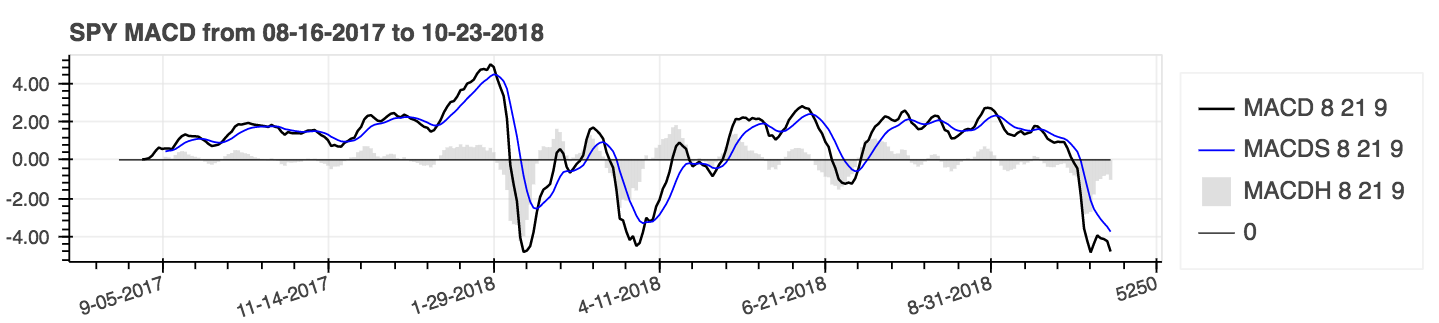 |
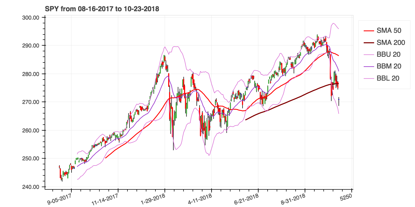
help(ta.ichimoku) .lookahead=False cae la columna Chikou Span para evitar una posible fuga de datos.| Promedios móviles simples (SMA) y Bollinger Bands (Bands) |
|---|
|
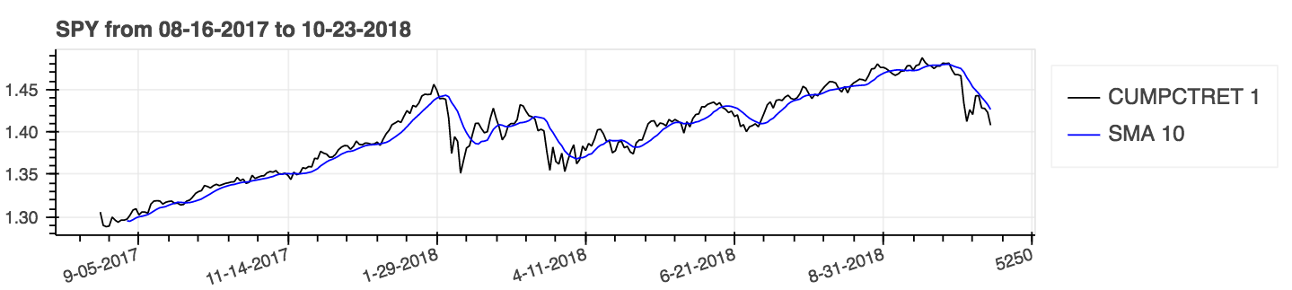
Use el parámetro: acumulativo = true para resultados acumulativos.
| Porcentaje de retorno (acumulativo) con un promedio móvil simple (SMA) |
|---|
 |
| Puntaje z |
|---|
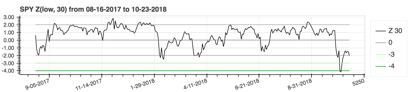 |
lookahead=False para deshabilitar el centrado y eliminar la posible fuga de datos.| Índice de movimiento direccional promedio (ADX) |
|---|
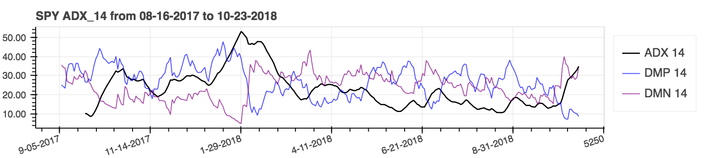 |
| Rango verdadero promedio (ATR) |
|---|
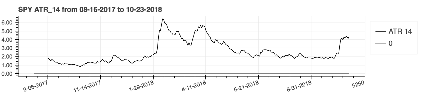 |
| Volumen en equilibrio (obv) |
|---|
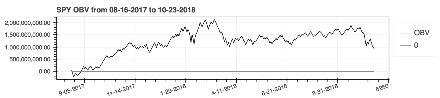 |
Las métricas de rendimiento son una nueva adición al paquete y, en consecuencia, probablemente no sean confiables. Use bajo su propio riesgo. Estas métricas devuelven un flotador y no forman parte de la extensión del marco de datos . Se llaman la forma estándar. Por ejemplo:
 import pandas_ta as ta
result = ta . cagr ( df . close ) Para una integración más fácil con el método de VectorBT from_signals , el método ta.trend_return se ha reemplazado con el método ta.tsignals para simplificar la generación de señales comerciales. Para un ejemplo completo, consulte el ejemplo de backtest vectorBT de Notebook de Jupyter con pandas TA en el directorio de ejemplos.
 import pandas as pd
import pandas_ta as ta
import vectorbt as vbt

df = pd . DataFrame (). ta . ticker ( "AAPL" ) # requires 'yfinance' installed

# Create the "Golden Cross"
df [ "GC" ] = df . ta . sma ( 50 , append = True ) > df . ta . sma ( 200 , append = True )

# Create boolean Signals(TS_Entries, TS_Exits) for vectorbt
golden = df . ta . tsignals ( df . GC , asbool = True , append = True )

# Sanity Check (Ensure data exists)
print ( df )

# Create the Signals Portfolio
pf = vbt . Portfolio . from_signals ( df . close , entries = golden . TS_Entries , exits = golden . TS_Exits , freq = "D" , init_cash = 100_000 , fees = 0.0025 , slippage = 0.0025 )

# Print Portfolio Stats and Return Stats
print ( pf . stats ())
print ( pf . returns_stats ())mamode Kwarg con más opciones de promedio móvil con la función de utilidad de promedio móvil ta.ma() . Para simplificar, todas las opciones son promedios móvil de fuente única. Esta es principalmente una utilidad interna utilizada por indicadores que tienen un mamode Kwarg . Esto incluye indicadores: AccBands , AMAT , AOBV , ATR , BBANDS , BIES , EFI , HILO , KC , NATR , QQE , RVI y TUMO ; Los parámetros mamode predeterminados no han cambiado. Sin embargo, el usuario también puede usar ta.ma() si es necesario. Para más información: help(ta.ma)to_utc , para convertir el índice DataFrame a UTC. Consulte: help(ta.to_utc) ahora como una propiedad Pandas TA DataFrame para convertir fácilmente el índice DataFrame en UTC. close > sma(close, 50) devuelve la tendencia, las entradas comerciales y las salidas comerciales de esa tendencia para que sea compatible con VectorBT al establecer asbool=True para obtener entradas y salidas comerciales booleanas. Ver help(ta.tsignals) help(ta.alma) Cuenta de negociación o fondo. Ver help(ta.drawdown)help(ta.cdl_pattern)help(ta.cdl_z)help(ta.cti)help(ta.xsignals)help(ta.dm)help(ta.ebsw)help(ta.jma)help(ta.kvo)help(ta.stc)help(ta.squeeze_pro)df.ta.strategy() por razones de rendimiento. Ver help(ta.td_seq)help(ta.tos_stdevall)help(ta.vhf) mamode de argumento renombrado al mode . Ver help(ta.accbands) .mamode con " RMA " predeterminado y con las mismas opciones mamode que TradingView. Nuevo argumento lensig para que se comporte como el indicador ADX Builtin de TradingView. Ver help(ta.adx) .drift agregado y nombres de columnas más descriptivos.mamode predeterminado ahora es " RMA " y con las mismas opciones mamode que TradingView. Ver help(ta.atr) .ddoff para controlar los grados de libertad. También incluyó el porcentaje de BB (BBP) como la columna final. El valor predeterminado es 0. Ver help(ta.bbands) .ln para usar logaritmo natural (verdadero) en lugar del logaritmo estándar (falso). El valor predeterminado es falso. Ver help(ta.chop) .tvmode agregado con verdadero True . Cuando tvmode=False , CKSP implementa "el nuevo operador técnico" con valores predeterminados. Ver help(ta.cksp) .talib utilizará la versión de TA lib y si se instala TA lib. El valor predeterminado es verdadero. Ver help(ta.cmo) .strict si la serie disminuye continuamente durante length del período con un cálculo más rápido. Predeterminado: False . El argumento percent también se ha agregado sin valor predeterminado. Ver help(ta.decreasing) .strict si la serie aumenta continuamente durante length del período con un cálculo más rápido. Predeterminado: False . El argumento percent también se ha agregado sin valor predeterminado. Ver help(ta.increasing) .help(ta.kvo) .as_strided o el nuevo método sliding_window_view . Esto debería resolver problemas con Google Colab y sus actualizaciones de dependencia tardía, así como las dependencias de Tensorflow, como se discutió en los problemas #285 y #329.asmode habilita como versión de MacD. El valor predeterminado es falso. Ver help(ta.macd) .sar de TradingView. Nuevo argumento af0 para inicializar el factor de aceleración. Ver help(ta.psar) .mamode de argumentos como una opción. El valor predeterminado es SMA para que coincida con TA lib. Ver help(ta.ppo) .signal agregada con el valor predeterminado 13 y mamode de modo MA de señal con EMA predeterminado como argumentos. Ver help(ta.tsi) .help(ta.vp) .help(ta.vwma) .anchor . Valor predeterminado: "D" para "Daily". Vea los alias de compensación de Timeseries para opciones adicionales. Requiere que el índice DataFrame sea un DateTimeIndex. Ver help(ta.vwap) .help(ta.vwma) .Z_length a ZS_length . Ver help(ta.zscore) .Ta-Lib original | TradingView | Gráfico de sierra | MQL5 | FM Labs | Código Pro Real | Usuario 42
¿Sentirse generoso, como el paquete o quiere ver que se convierta en un paquete más maduro?


