cufflinks

Manset

Perpustakaan ini mengikat kekuatan plot dengan fleksibilitas panda untuk merencanakan dengan mudah.

Perpustakaan ini tersedia di https://github.com/santosjorge/cufflinks

Tutorial ini mengasumsikan bahwa kredensial pengguna yang diplot telah dikonfigurasi sebagaimana dinyatakan pada panduan memulai.

Tutorial:

• Galeri Bagan
• Panda menyukai visualisasi
• Dasar -dasarnya
• Manajemen warna
• Mode offline

Catatan Rilis

V0.17.0

Dukungan untuk plotly 4.x
Manset tidak lagi kompatibel dengan plotly 3.x

V0.14.0

Dukungan untuk Plotly 3.0

V0.13.0

Pembantu iplot Baru. Untuk melihat daftar parameter yang komprehensif CF.help ()

 # For a list of supported figures
cf . help ()
# Or to see the parameters supported that apply to a given figure try
cf . help ( 'scatter' )
cf . help ( 'candle' ) #etc

V0.12.0

Dibelingkangi dependen pada ta-lib. Perpustakaan ini tidak lagi diperlukan. Semua studi telah ditulis ulang di Python.

V0.11.0

• QuantFigure adalah kelas baru yang akan menghasilkan objek grafik dengan kegigihan. Parameter dapat ditambahkan/dimodifikasi pada titik tertentu.

Ini bisa semudah:

 df = cf . datagen . ohlc ()
qf = cf . QuantFig ( df , title = 'First Quant Figure' , legend = 'top' , name = 'GS' )
qf . add_bollinger_bands ()
qf . iplot ()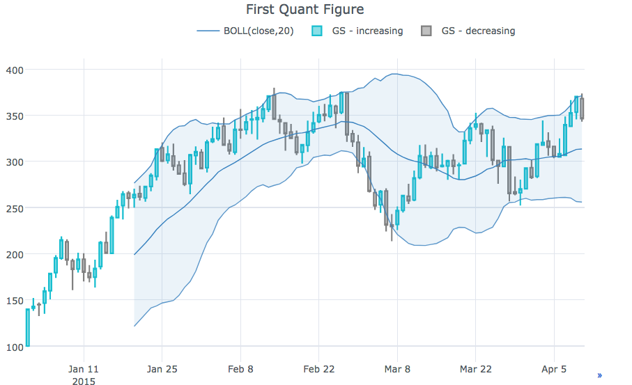

• Studi analisis teknis dapat ditambahkan berdasarkan permintaan.

 qf . add_sma ([ 10 , 20 ], width = 2 , color = [ 'green' , 'lightgreen' ], legendgroup = True )
qf . add_rsi ( periods = 20 , color = 'java' )
qf . add_bollinger_bands ( periods = 20 , boll_std = 2 , colors = [ 'magenta' , 'grey' ], fill = True )
qf . add_volume ()
qf . add_macd ()
qf . iplot ()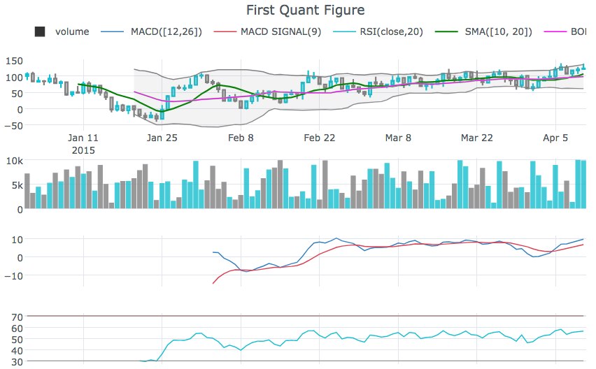

V0.10.0

• rangeslider untuk menampilkan slider rentang tanggal di bagian bawah
  • cf.datagen.ohlc().iplot(kind='candle',rangeslider=True)
• rangeselector untuk menampilkan tombol untuk mengubah rentang tanggal yang ditampilkan
  • cf.datagen.ohlc(500).iplot(kind='candle', rangeselector={ 'steps':['1y','2 months','5 weeks','ytd','2mtd','reset'], 'bgcolor' : ('grey',.3), 'x': 0.3 , 'y' : 0.95})
• Kustomisasi Anntions, dengan fontsize , fontcolor , textangle
  • Mode Label
    • cf.datagen.lines(1,mode='stocks').iplot(kind='line', annotations={'2015-02-02':'Market Crash', '2015-03-01':'Recovery'}, textangle=-70,fontsize=13,fontcolor='grey')
  • Mode eksplisit
    • cf.datagen.lines(1,mode='stocks').iplot(kind='line', annotations=[{'text':'exactly here','x':'0.2', 'xref':'paper','arrowhead':2, 'textangle':-10,'ay':150,'arrowcolor':'red'}])

V0.9.0

• Figure.iplot() untuk plot angka
• Lilin berkinerja tinggi dan plot OHLC baru
  • cf.datagen.ohlc().iplot(kind='candle')

V0.8.0

• 'cf.datagen.choropleth ()' untuk untuk data choropleth sampel.
• 'cf.datagen.scattergeo ()' untuk untuk data scattergeo sampel.
• Dukungan untuk tokoh choropleth dan scattergeo di iplot
• 'cf.get_colorscale' untuk peta dan objek plot yang mendukung ColorsCales

V0.7.1

• xrange , yrange dan zrange dapat ditentukan dalam iplot dan getLayout
  • cf.datagen.lines(1).iplot(yrange=[5,15])
• layout_update dapat diatur di iplot dan getLayout untuk secara eksplisit memperbarui nilai Layout apa pun

V0.7

• Dukungan untuk Python 3

v0.6

Lihat Notebook Ipython

• Dukungan untuk diagram lingkaran
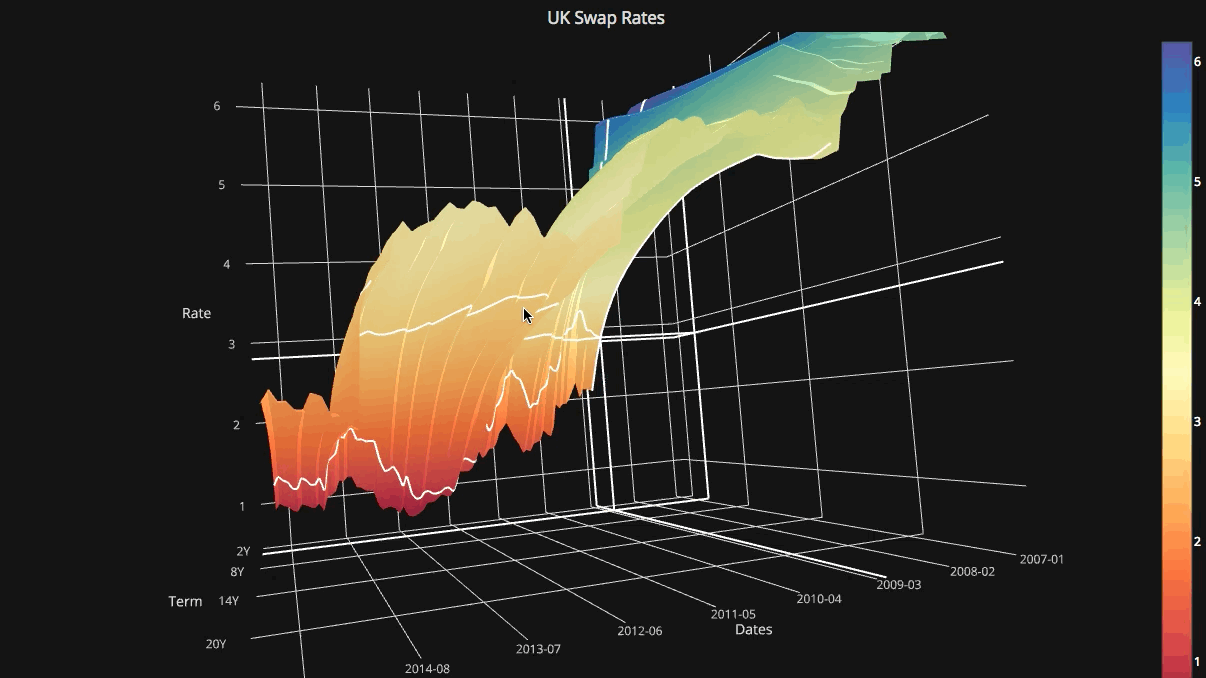
  • cf.datagen.pie().iplot(kind='pie',labels='labels',values='values')
• Hasilkan data terbuka, tinggi, rendah, tutup
  • datagen.ohlc()
• Dukungan Bagan Lilin
  • ohlc=cf.datagen.ohlc()
ohlc.iplot(kind='candle',up_color='blue',down_color='red')
• Dukungan OHLC (BAR)
  • ohlc=cf.datagen.ohlc()
ohlc.iplot(kind='ohlc',up_color='blue',down_color='red')
• Dukungan untuk Bagan Logaritmik (Logx | Logy)
  • df=pd.DataFrame([x**2] for x in range(100))
df.iplot(kind='lines',logy=True)
• Dukungan untuk MulitIndex DataFrames
• Dukungan untuk bilah kesalahan (error_x | error_y)
  • cf.datagen.lines(1,5).iplot(kind='bar',error_y=[1,2,3.5,2,2])
  • cf.datagen.lines(1,5).iplot(kind='bar',error_y=20, error_type='percent')
• Dukungan untuk Bilah Kesalahan Berkelanjutan
  • cf.datagen.lines(1).iplot(kind='lines',error_y=20,error_type='continuous_percent')
  • cf.datagen.lines(1).iplot(kind='lines',error_y=10,error_type='continuous',color='blue')
• Studi Analisis Teknis untuk Timeseries (Beta)
  • Rata -rata bergerak sederhana (SMA)
    • cf.datagen.lines(1,500).ta_plot(study='sma',periods=[13,21,55])
  • Indikator Kekuatan Relatif (RSI)
    • cf.datagen.lines(1,200).ta_plot(study='boll',periods=14)
  • Bollinger Bands (Boll)
    • cf.datagen.lines(1,200).ta_plot(study='rsi',periods=14)
  • Divergence konvergensi rata -rata bergerak (MACD)
    • cf.datagen.lines(1,200).ta_plot(study='macd',fast_period=12,slow_period=26, signal_period=9)

v0.5

• Dukungan grafik offline
  • cf.go_offline()
  • cf.go_online()
  • cf.iplot(figure,online=True) (untuk memaksa online saat dalam mode offline)
• Dukungan untuk poros sekunder
  • fig=cf.datagen.lines(3,columns=['a','b','c']).figure()
fig=fig.set_axis('b',side='right')
cf.iplot(fig)

V0.4

• Dukungan untuk Pengaturan Tema Global
  • cufflinks.set_config_file(theme='pearl')
• Tema baru ggplot
  • cufflinks.datagen.lines(5).iplot(theme='ggplot')
• Dukungan untuk grafik batang horizontal Barh
  • cufflinks.datagen.lines(2).iplot(kind='barh',barmode='stack',bargap=.1)
• Dukungan untuk orientasi histogram dan normalisasi
  • cufflinks.datagen.histogram().iplot(kind='histogram',orientation='h',norm='probability')
• Dukungan untuk plot area
  • cufflinks.datagen.lines(4).iplot(kind='area',fill=True,opacity=1)
• Dukungan untuk subplot
  • cufflinks.datagen.histogram(4).iplot(kind='histogram',subplots=True,bins=50)
  • cufflinks.datagen.lines(4).iplot(subplots=True,shape=(4,1),shared_xaxes=True,vertical_spacing=.02,fill=True)
• Dukungan untuk matriks pencar untuk menampilkan distribusi di antara setiap seri di DataFrame
  • cufflinks.datagen.lines(4,1000).scatter_matrix()
• Dukungan untuk Vline dan Hline untuk garis horizontal dan vertikal
  • cufflinks.datagen.lines(3).iplot(hline=[2,3])
  • cufflinks.datagen.lines(3).iplot(hline=dict(y=2,color='blue',width=3))
• Dukungan untuk VSPAN dan HSPAN untuk area horizontal dan vertikal
  • cufflinks.datagen.lines(3).iplot(hspan=(-1,2))
  • cufflinks.datagen.lines(3).iplot(hspan=dict(y0=-1,y1=2,color='orange',fill=True,opacity=.4))

v0.3.2

• Pengaturan Global untuk Bagan Publik
  • cufflinks.set_config_file(world_readable=True)

v0.3

• Grafik spread yang ditingkatkan
  • cufflinks.datagen.lines(2).iplot(kind='spread')
• Dukungan untuk grafik Heatmap
  • cufflinks.datagen.heatmap().iplot(kind='heatmap')
• Dukungan untuk Grafik Gelembung
  • cufflinks.datagen.bubble(4).iplot(kind='bubble',x='x',y='y',text='text',size='size',categories='categories')
• Dukungan untuk grafik Bubble3D
  • cufflinks.datagen.bubble3d(4).iplot(kind='bubble3d',x='x',y='y',z='z',text='text',size='size',categories='categories')
• Dukungan untuk grafik kotak
  • cufflinks.datagen.box().iplot(kind='box')
• Dukungan untuk bagan permukaan
  • cufflinks.datagen.surface().iplot(kind='surface')
• Dukungan untuk grafik sebar
  • cufflinks.datagen.scatter3d().iplot(kind='scatter3d',x='x',y='y',z='z',text='text',categories='categories')
• Dukungan untuk histogram
  • cufflinks.datagen.histogram(2).iplot(kind='histogram')
• Pembuatan data untuk jenis plot yang paling umum
  • cufflinks.datagen
• Ekstraksi data: Ekstrak data dari grafik plotty apa pun. Data disampaikan di DataFrame
  • cufflinks.to_df(Figure)
• Integrasi dengan colorlover
  • Dukungan untuk skala iplot(colorscale='accent') untuk memplot grafik menggunakan skala warna aksen
  • cufflinks.scales () untuk melihat semua skala yang tersedia
• Dukungan untuk Warna bernama * iplot(colors=['pink','red','yellow'])