Huawei UK University Challenge Competition 2021
1.0.0

团队主持人: Kahraman Kostas
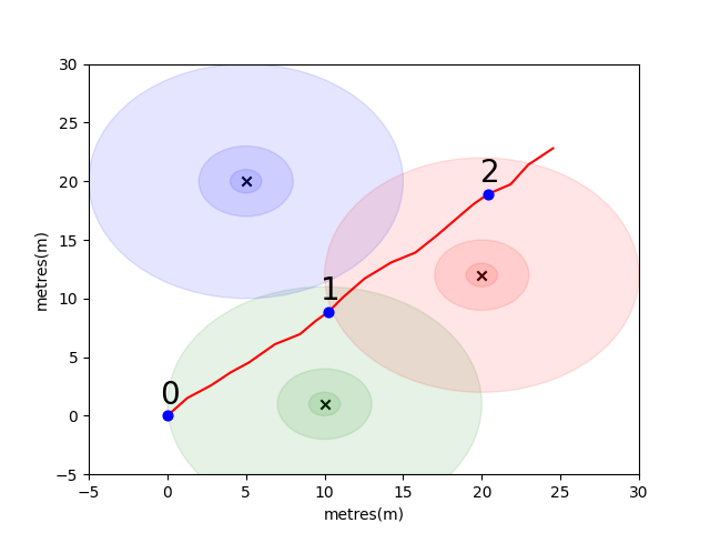
为了让您开始,我们已经解决了一个简单的问题,以引入一些关键的室内定位概念。考虑以下环境:在有3个WiFi发射器的情况下,用户正在开放空间中行驶(我们将本用户创建的数据称为轨迹)。每个发射器都有一个唯一的MAC地址。用户配备了一款智能手机,该智能手机将定期扫描WiFi环境并记录每个检测到的Mac(以DB)的RSSI。
对于此模型,我们为每个发射器使用了标准的日志自由空间传播模型。这是一个简单的模型,可在自由空间中效果很好,但是在带有墙壁和其他障碍物的实际室内环境中分解,可以以更复杂的方式反弹信号。通常,随着发射天线的固定能量分布在增加的区域,随着波浪的传播,我们确实希望RSSI在距离上急剧下降。在下面的图中,每个圆表示下降的10dB。
用户从点(0,0)上向东北行走,那里的电话进行了三个环境扫描。每次扫描记录的数据如下所示。
 scan 0 -> {'green': -60, 'blue': -66, 'red': -67}
scan 1 -> {'green': -58, 'blue': -61, 'red': -60}
scan 2 -> {'green': -66, 'blue': -62, 'red': -59}
WiFi环境的复杂且本地独特的特性使其对于室内定位系统非常有用。例如,在下图中,图像scan 1在三个发射器的质心上测量数据,并且在这种环境中没有其他位置可以进行读取相似的RSSI值。考虑到来自独立轨迹的一组扫描或“指纹”,我们有兴趣计算它们在WiFi空间中的相似程度,因为这表明它们在真实空间中的距离有多近。
您的第一个挑战是编写一个函数,以计算我们上面引入的样品轨迹中的每个扫描之间的欧几里得距离和曼哈顿距离指标。使用来自单个轨迹的数据是测试相似性度量质量的好方法,因为我们可以使用手机的互助测量单元(IMU)获得相当准确的真实距离估算,该数据由行人死亡估算使用,该单元使用该数据(PDR)模块。
 def euclidean ( fp1 , fp2 ):
    raise NotImplementedError

def manhattan ( fp1 , fp2 ):
    raise NotImplementedError
# solution of the above functions
from scipy . spatial import distance
def euclidean ( fp1 , fp2 ):
fp1 = list ( fp1 . values ())
fp2 = list ( fp2 . values ())
return distance . euclidean ( fp1 , fp2 )
def manhattan ( fp1 , fp2 ):
fp1 = list ( fp1 . values ())
fp2 = list ( fp2 . values ())
return distance . cityblock ( fp1 , fp2 ) import json
import numpy as np
import matplotlib . pyplot as plt
from metrics import eval_dist_metric
with open ( "intro_trajectory_1.json" ) as f :
traj = json . load ( f )
## Pre-calculate the pair indexes we are interested in
keys = []
for fp1 in traj [ 'fps' ]:
for fp2 in traj [ 'fps' ]:
# only calculate the upper triangle
if fp1 [ 'step_index' ] > fp2 [ 'step_index' ]:
keys . append (( fp1 [ 'step_index' ], fp2 [ 'step_index' ]))
## Get the distances from PDR
true_d = {}
for step1 in traj [ 'steps' ]:
for step2 in traj [ 'steps' ]:
key = ( step1 [ 'step_index' ], step2 [ 'step_index' ])
if key in keys :
true_d [ key ] = abs ( step1 [ 'di' ] - step2 [ 'di' ])
euc_d = {}
man_d = {}
for fp1 in traj [ 'fps' ]:
for fp2 in traj [ 'fps' ]:
key = ( fp1 [ 'step_index' ], fp2 [ 'step_index' ])
if key in keys :
euc_d [ key ] = euclidean ( fp1 [ 'profile' ], fp2 [ 'profile' ])
man_d [ key ] = manhattan ( fp1 [ 'profile' ], fp2 [ 'profile' ])
print ( "Euclidean Average Error" )
print ( f' { eval_dist_metric ( euc_d , true_d ):.2f } ' )
print ( "Manhattan Average Error" )
print ( f' { eval_dist_metric ( man_d , true_d ):.2f } ' ) Euclidean Average Error
9.29
Manhattan Average Error
4.90
如果您正确地实施了功能,则应该看到欧几里得公制的平均误差为9.29 ,而曼哈顿仅为4.90 。 So for this data, the Manhattan distance is a better estimate of the true distance.
This is of course a very simplistic model.确实,以这种方式,RSSI值与自由空间距离之间没有直接的关系。 Typically, when we create our own estimates for distance we would use the known pdr distances from within a trajectory to fit the numeric score to a physical distance estimate.
For your main challenge, we would like you to develop your own metric to estimate the real-world distance between two scans, based solely on their WiFi fingerprints. We will provide you with real crowdsourced data collected early in 2021 from a single mall. The data will contain 114661 fingerprints scans and 879824 distances between the scans.距离将是我们将考虑的其他信息的最佳估计。
我们将提供一组指纹对的测试集,您需要编写一个函数,告诉我们它们的相距多远。
该功能可能就像我们上面介绍的一个指标之一一样简单,也可以像完整的机器学习解决方案一样复杂,该解决方案在不同情况下学会了对不同的MAC地址(或MAC地址组合)的加权不同。
要考虑的一些最后点:
数据将作为您的三个文件组装。
task1_fingerprints.json包含问题的所有指纹信息。 That is each entry represents a real scan of the WiFi emitters in an area of the mall.您会发现许多指纹中都会存在相同的MAC地址。
The task1_train.csv contains the valid training pairs to help you design/train your algorithm.每个id1-id2对具有一个标记的地面真相距离(以米为单位),每个ID对应于task1_fingerprints.json的指纹。
task1_test.csv格式与task1_train.csv格式相同,但没有包含的位移。这些是我们希望您使用原始指纹信息预测的内容。
 import csv
import json
import os
from tqdm import tqdm

path_to_data = "for_contestants"

with open ( os . path . join ( path_to_data , "task1_fingerprints.json" )) as f :
    fps = json . load ( f )

with open ( os . path . join ( path_to_data , "task1_train.csv" )) as f :
    train_data = []
    train_h = csv . DictReader ( f )
    for pair in tqdm ( train_h ):
        train_data . append ([ pair [ 'id1' ], pair [ 'id2' ], float ( pair [ 'displacement' ])])

with open ( os . path . join ( path_to_data , "task1_test.csv" )) as f :
    test_h = csv . DictReader ( f )
    test_ids = []
    for pair in tqdm ( test_h ):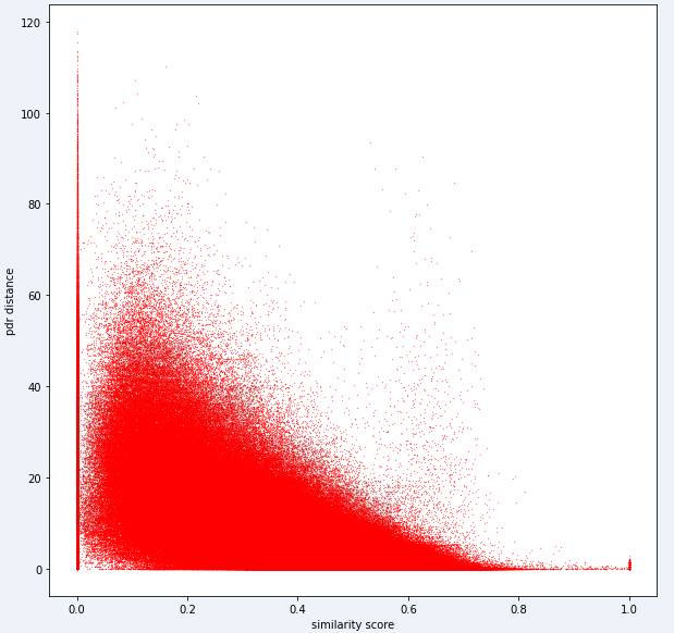
test_ids . append ([ pair [ 'id1' ], pair [ 'id2' ]])最终,理想的模型应该能够在高度尺寸的指纹空间(1指纹可以包含许多测量值)和1维距离空间之间找到精确的映射。将PDR距离(与培训数据)绘制在某些计算的相似性度量上,以查看该度量是否揭示出明显的趋势可能是有用的。高相似性应与低距离相关。
以下是我们内部用于此任务的一个距离指标。您可以看到,即使对于这个指标,我们也有大量的噪音。
由于这种噪音水平,我们的任务1的评分指标将偏向于精确度而不是召回
您的提交应使用test1_test.csv文件中的确切ID,并应使用该指纹对的估计距离(以米为单位)填充第三个(当前空)位移列。
 def my_distance_function ( fp1 , fp2 ):
    raise NotImplementedError
output_data = [[ "id1" , "id2" , "displacement" ]]
for id1 , id2 in tqdm ( test_ids ):
fp1 = fps [ id1 ]
fp2 = fps [ id2 ]
distance_estimate = my_distance_function ( fp1 , fp2 )
output_data . append ([ id1 , id2 , distance_estimate ])
with open ( "MySubmission.csv" , "w" , newline = '' ) as f :
writer = csv . writer ( f )
writer . writerows ( output_data )第一个任务中的步骤可以汇总如下。
这些步骤在下图中说明。
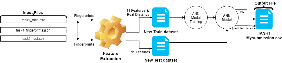
我们使用Python 3.6.5创建应用程序文件。我们包括了一些其他模块,这些模块未包含在比赛开始时给出的示例文件中。这些模块可以列为:
| molules | 任务 |
|---|---|
| 张量 | 深度学习 |
| 熊猫 | 数据分析 |
| Scipy | 距离计算 |
We started with the installation of these modules as the first step.
 ## 1.1 Installing modules
!p ip install tensorflow == 2.6 . 2
!p ip install scipy
!p ip install pandas In this step, we fixed the related random seed to be used in order to obtain repeatable results. In this way, we have provided a deterministic path where we get the same result in every run.但是,根据我们的观察,用不同计算机获得的结果可能略有不同(±1%)
 ## 1.2  Setting Random Seeds
seed_value = 0

import os
os . environ [ 'PYTHONHASHSEED' ] = str ( seed_value )

import random
random . seed ( seed_value )

import numpy as np
np . random . seed ( seed_value )

import tensorflow as tf
tf . random . set_seed ( seed_value )

import tensorflow as tf

session_conf = tf . compat . v1 . ConfigProto ( intra_op_parallelism_threads = 1 , inter_op_parallelism_threads = 1 )
sess = tf . compat . v1 . Session ( graph = tf . compat . v1 . get_default_graph (), config = session_conf )在本节中,我们加载了将使用的数据。我们从给出的示例文件( Task1-IPS-Challenge-2021.ipynb )中获取了代码和说明。
task1_fingerprints.json包含问题的所有指纹信息。那就是每个条目代表购物中心区域中WiFi发射器的真实扫描。您会发现许多指纹中都会存在相同的MAC地址。
task1_train.csv包含有效的培训对,以帮助您设计/训练算法。每个id1-id2对具有一个标记的地面真相距离(以米为单位),每个ID对应于task1_fingerprints.json的指纹。
task1_test.csv格式与task1_train.csv格式相同,但没有包含的位移。
 ## 1.3 Loading the data
import csv
import json
import os
from tqdm import tqdm

path_to_data = "for_contestants"

with open ( os . path . join ( path_to_data , "task1_fingerprints.json" )) as f :
    fps = json . load ( f )

with open ( os . path . join ( path_to_data , "task1_train.csv" )) as f :
    train_data = []
    train_h = csv . DictReader ( f )
    for pair in tqdm ( train_h ):
        train_data . append ([ pair [ 'id1' ], pair [ 'id2' ], float ( pair [ 'displacement' ])])

with open ( os . path . join ( path_to_data , "task1_test.csv" )) as f :
    test_h = csv . DictReader ( f )
    test_ids = []
    for pair in tqdm ( test_h ):
        test_ids . append ([ pair [ 'id1' ], pair [ 'id2' ]])
879824it [05:16, 2778.31it/s]
5160445it [01:00, 85269.27it/s]
在此步骤中,我们使用两个功能执行特征提取。 feature_extraction_file函数只需从JSON文件中拉出指纹的相关值(成对),然后将它们发送到feature_extraction函数以进行计算。
在feature_extraction函数中,如果这两个指纹在尺寸和所包含的设备方面相互不同,则将两个指纹中包含的所有设备汇集在一起以形成一个常见的序列而无需重复。 In each array, we make these two arrays identical (in terms of devices they include) by assigning the value 0 to the non-corresponding devices.以下图像中的一个示例对此过程进行了解释。
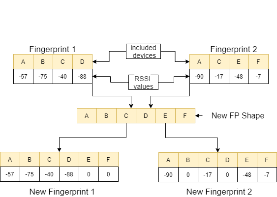
这两个指纹之间的距离使用11种不同的方法进行了计算[1]。这些方法是:
然后,将这些值定向到feature_extraction_file函数,并在此函数中保存为CSV文件。换句话说,由于此过程,各种尺寸的指纹变成了11-曲的CSV文件。使用这些新创建的功能对要使用的模型进行了训练和测试。
 ## 1.4 Feature Extraction

def feature_extraction_file ( data , name , flag ):
    features = [[ "braycurtis" ,
    "canberra" ,
    "chebyshev" ,
    "cityblock" ,
    "correlation" ,
    "cosine" ,
    "euclidean" ,
    "jensenshannon" ,
    "minkowski" ,
    "sqeuclidean" ,
    "wminkowski" , "real" ]]
    for i in tqdm (( data ), position = 0 , leave = True ):
        fp1 = fps [ i [ 0 ]]
        fp2 = fps [ i [ 1 ]]
        feature = feature_extraction ( fp1 , fp2 )
        if flag :
            feature . append ( i [ 2 ])
        else : feature . append ( 0 )
        features . append ( feature )
    with open ( name , "w" , newline = '' ) as f :
        writer = csv . writer ( f )
        writer . writerows ( features )
    #print(features)
## 1.4 Feature Extraction
def feature_extraction ( fp1 , fp2 ):
mac = set ( list ( fp1 . keys ()) + list ( fp2 . keys ()))
mac = { i : 0 for i in mac }
f1 = mac . copy ()
f2 = mac . copy ()
for key in fp1 :
f1 [ key ] = fp1 [ key ]
for key in fp2 :
f2 [ key ] = fp2 [ key ]
f1 = list ( f1 . values ())
f2 = list ( f2 . values ())
braycurtis = scipy . spatial . distance . braycurtis ( f1 , f2 )
canberra = scipy . spatial . distance . canberra ( f1 , f2 )
chebyshev = scipy . spatial . distance . chebyshev ( f1 , f2 )
cityblock = scipy . spatial . distance . cityblock ( f1 , f2 )
correlation = scipy . spatial . distance . correlation ( f1 , f2 )
cosine = scipy . spatial . distance . cosine ( f1 , f2 )
euclidean = scipy . spatial . distance . euclidean ( f1 , f2 )
jensenshannon = scipy . spatial . distance . jensenshannon ( f1 , f2 )
minkowski = scipy . spatial . distance . minkowski ( f1 , f2 )
sqeuclidean = scipy . spatial . distance . sqeuclidean ( f1 , f2 )
wminkowski = scipy . spatial . distance . wminkowski ( f1 , f2 , 1 , np . ones ( len ( f1 )))
output_data = [ braycurtis ,
canberra ,
chebyshev ,
cityblock ,
correlation ,
cosine ,
euclidean ,
jensenshannon ,
minkowski ,
sqeuclidean ,
wminkowski ]
output_data = [ 0 if x != x else x for x in output_data ]
return output_data 在此任务中,有指纹扫描,这些扫描具有来自购物中心WiFi发射器周围环境的RRSI信号。首先,挑战希望我们估计两种指纹扫描之间的距离,这是回归任务。我们使用了受生物神经网络启发的ANN(人工神经网络)。安由三层组成;输入层,隐藏图层(多个)和输出层。 ANN从输入层开始,其中包括训练数据(带有功能),将数据传递到第一个隐藏层,该隐藏层由第一个隐藏层的权重计算出数据。在隐藏的层中,重量的重量计算到输入中,然后将它们应用于激活函数[2]。由于我们的问题是回归,我们的最后一层是一个单个输出神经元:其输出是指纹扫描对之间的距离。我们的第一个隐藏层具有64个,第二层具有128个神经元。该模型的所有架构如下。 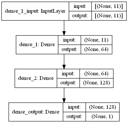
我们使用两个功能进行深度学习。create_model create_model塑造了训练数据以训练模型并确定模型的结构。 model_features函数可产生具有指定结构的模型。通过create_model函数训练后,可以保存创建的模型。
## 1.5 Model
import scipy . spatial
import pandas as pd
import numpy as np
import matplotlib . pyplot as plt
from tensorflow import keras
from tensorflow . keras . models import Sequential
from tensorflow . keras . layers import Dense
#from keras.utils.vis_utils import plot_model
% matplotlib inline
def model_features ( i , ii ):
model = Sequential ()
model . add ( Dense ( i , input_shape = ( 11 , ), activation = 'relu' , name = 'dense_1' ))
model . add ( Dense ( ii , activation = 'relu' , name = 'dense_2' ))
model . add ( Dense ( 1 , activation = 'linear' , name = 'dense_output' ))
model . compile ( optimizer = 'adam' , loss = 'mse' , metrics = [ 'mae' ])
model . summary ()
#plot_model(model, to_file='model_plot.png', show_shapes=True, show_layer_names=True)
#print(model.get_config())
return model
def create_model ( name ):
df = pd . read_csv ( name )
df . replace ([ np . inf , - np . inf ], np . nan , inplace = True )
df = df . fillna ( 0 )
X = df [ df . columns [ 0 : - 1 ]]
X_train = np . array ( X )
y_train = np . array ( df [ df . columns [ - 1 ]])
model = model_features ( 64 , 128 )
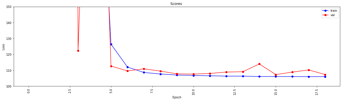
history = model . fit ( X_train , y_train , epochs = 19 , validation_split = 0.5 ) #,batch_size=1)
loss = history . history [ 'loss' ]
val_loss = history . history [ 'val_loss' ]
my_xticks = list ( range ( len ( loss )))
plt . figure ( figsize = ( 20 , 5 ))
plt . plot ( my_xticks , loss , linestyle = '-' , marker = 'o' , color = 'b' , label = "train" )
plt . plot ( my_xticks , val_loss , linestyle = '-' , marker = 'o' , color = 'r' , label = "val" )
plt . title ( "Scores " )
plt . legend ( numpoints = 1 )
plt . ylabel ( "Loss" )
plt . xlabel ( "Epoch" )
plt . xticks ( rotation = 90 )
plt . ylim ([ 100 , 150 ])
plt . show ()
madelname = "./THEMODEL"
model . save ( madelname )
print ( "Model Created!" )
此功能检查训练和测试数据是否通过功能提取。如果没有,它可以通过调用相应的功能来创建这些文件和模型。处理模型和所有特征提取后,它将测试数据格式化以产生最终结果。
 ## 1.6 Checking the inputs
from numpy import inf
from numpy import nan

def create_new_files ( train , test ):
    model_path = "./THEMODEL/"
    my_train_file = 'new_train_features.csv'
    my_test_file = 'new_test_features.csv'


    if os . path . isfile ( my_train_file ) :
        pass
    else :

        print ( "Please wait! Training data feature extraction is in progress... n it will take about 10 minutes" )
        feature_extraction_file ( train , my_train_file , 1 )
        print ( "TThe training feature extraction completed!!!" )


    if os . path . isfile ( my_test_file ) :
        pass
    else :

        print ( "Please wait! Testing data feature extraction is in progress... n it will take about 100-120 minutes" )
        feature_extraction_file ( test , my_test_file , 0 )
        print ( "The testing feature extraction completed!!!" )


    if  os . path . isdir ( model_path ):
        pass
    else :

        print ( "Please wait! Creating the deep learning model... n it will take about 10 minutes" )
        create_model ( my_train_file )
        print ( "The model file created!!! n n n " )

    model = keras . models . load_model ( model_path )
    df = pd . read_csv ( my_test_file )
    df . replace ([ np . inf , - np . inf ], np . nan , inplace = True )
    df = df . fillna ( 0 )
    X_train = df [ df . columns [ 0 : - 1 ]]
    X_train = np . array ( X_train )
    y_train = np . array ( df [ df . columns [ - 1 ]])
    predicted = model . predict ( X_train )
    print ( "Please wait! Creating resuşts... " )

return predicted 此步骤触发器具有提取和模型创建过程,并允许所有过程开始。因此,使用test1_test.csv文件中的ID填充该指纹对的第三个(位移)列,并将此文件保存在目录中,并使用名称TASK1-MySubmission.csv 。
 ## 1.7 Submission
distance_estimate = create_new_files ( train_data , test_ids )
count = 0

output_data = [[ "id1" , "id2" , "displacement" ]]
for id1 , id2 in tqdm ( test_ids ):
    output_data . append ([ id1 , id2 , distance_estimate [ count ][ 0 ]])
    count += 1
print ( "Process finished. Preparing result file ..." )
with open ( "TASK1-MySubmission.csv" , "w" , newline = '' ) as f :
    writer = csv . writer ( f )
    writer . writerows ( output_data )
print ( "The results are ready. n See MySubmission.csv" )
Please wait! Creating the deep learning model...
it will take about 10 minutes
Model: "sequential_3"
_________________________________________________________________
Layer (type) Output Shape Param #
=================================================================
dense_1 (Dense) (None, 64) 768
_________________________________________________________________
dense_2 (Dense) (None, 128) 8320
_________________________________________________________________
dense_output (Dense) (None, 1) 129
=================================================================
Total params: 9,217
Trainable params: 9,217
Non-trainable params: 0
_________________________________________________________________
Epoch 1/19
13748/13748 [==============================] - 30s 2ms/step - loss: 2007233.6250 - mae: 161.3013 - val_loss: 218.8822 - val_mae: 11.5630
Epoch 2/19
13748/13748 [==============================] - 27s 2ms/step - loss: 24832.6309 - mae: 53.9385 - val_loss: 123437.0859 - val_mae: 307.2885
Epoch 3/19
13748/13748 [==============================] - 26s 2ms/step - loss: 4028.0859 - mae: 29.9960 - val_loss: 3329.2024 - val_mae: 49.9126
Epoch 4/19
13748/13748 [==============================] - 27s 2ms/step - loss: 904.7919 - mae: 17.6284 - val_loss: 122.3358 - val_mae: 6.8169
Epoch 5/19
13748/13748 [==============================] - 25s 2ms/step - loss: 315.7050 - mae: 11.9098 - val_loss: 404.0973 - val_mae: 15.2033
Epoch 6/19
13748/13748 [==============================] - 26s 2ms/step - loss: 126.3843 - mae: 7.8173 - val_loss: 112.6499 - val_mae: 7.6804
Epoch 7/19
13748/13748 [==============================] - 27s 2ms/step - loss: 112.0149 - mae: 7.4220 - val_loss: 109.5987 - val_mae: 7.1964
Epoch 8/19
13748/13748 [==============================] - 26s 2ms/step - loss: 108.6342 - mae: 7.3271 - val_loss: 110.9016 - val_mae: 7.6862
Epoch 9/19
13748/13748 [==============================] - 26s 2ms/step - loss: 107.6721 - mae: 7.2827 - val_loss: 109.5083 - val_mae: 7.5235
Epoch 10/19
13748/13748 [==============================] - 27s 2ms/step - loss: 107.0110 - mae: 7.2290 - val_loss: 107.7498 - val_mae: 7.1105
Epoch 11/19
13748/13748 [==============================] - 29s 2ms/step - loss: 106.7296 - mae: 7.2158 - val_loss: 107.6115 - val_mae: 7.1178
Epoch 12/19
13748/13748 [==============================] - 26s 2ms/step - loss: 106.5561 - mae: 7.2039 - val_loss: 107.9937 - val_mae: 6.9932
Epoch 13/19
13748/13748 [==============================] - 26s 2ms/step - loss: 106.3344 - mae: 7.1905 - val_loss: 108.8941 - val_mae: 7.4530
Epoch 14/19
13748/13748 [==============================] - 27s 2ms/step - loss: 106.3188 - mae: 7.1927 - val_loss: 109.0832 - val_mae: 7.5309
Epoch 15/19
13748/13748 [==============================] - 27s 2ms/step - loss: 106.1150 - mae: 7.1829 - val_loss: 113.9741 - val_mae: 7.9496
Epoch 16/19
13748/13748 [==============================] - 26s 2ms/step - loss: 106.0676 - mae: 7.1788 - val_loss: 107.2984 - val_mae: 7.2192
Epoch 17/19
13748/13748 [==============================] - 27s 2ms/step - loss: 106.0614 - mae: 7.1733 - val_loss: 108.8553 - val_mae: 7.4640
Epoch 18/19
13748/13748 [==============================] - 28s 2ms/step - loss: 106.0113 - mae: 7.1790 - val_loss: 110.2068 - val_mae: 7.6562
Epoch 19/19
13748/13748 [==============================] - 27s 2ms/step - loss: 106.0519 - mae: 7.1791 - val_loss: 107.3276 - val_mae: 7.0981
 INFO:tensorflow:Assets written to: ./THEMODELassets
Model Created!
The model file created!!!


Please wait! Creating resuşts...


100%|████████████████████████████████████████████████████████████████████| 5160445/5160445 [00:08<00:00, 610910.29it/s]


Process finished. Preparing result file ...
The results are ready.
 See MySubmission.csv
鉴于我们现在有一个用于评估WiFi距离的度量,但我们强烈建议一种图形聚类方法。
将数据中的每个WiFi指纹视为图中的节点,并且我们可以通过评估任何两个指纹的相似性来与图中的其他指纹形成边缘。我们可以为指纹之间具有很高相似性的边缘分配高的重量,而在不相似的边缘之间具有很高的相似性和低重量(或没有边缘)。从理论上讲,一个完全准确的相似性度量标准将在地板上微不足道地分开,因为我们可以排除大于4米(大约是建筑物1层的高度)的所有边缘。实际上,我们很可能会在楼层之间做出虚假的边缘,我们需要以某种方式打破这些边缘。
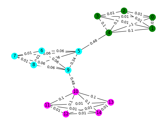
让我们从一个简单的示例开始。考虑下面的图表,其中节点颜色显示指纹的真实地板分类,边缘反映出我们认为这些节点存在于同一地板上。在此练习中,我们已经预先标记了每个边缘的“中间分数”,该度量可以计算出图形中任何两个节点之间的最短路径来计算该边缘的次数。通常,这将揭示表明高连通性的边缘,并且可能是去除的候选者。
在此示例中,使用边缘之间的分数来检测图形通信。 Return a list of lists where each sublist contains the node ids of the communities.请注意,这仅仅是为了帮助您理解问题,并且不计算实际解决方案。
 def detect_communities ( Graph ):
    ## This function should return a list of lists containing
    ## the node ids of the communities that you have detected.

    eb_score = nx . edge_betweenness_centrality ( G )

    raise NotImplementedError
import networkx as nx
from metrics import check_result
G = nx . read_adjlist ( "graph.adjlist" )
communities = detect_communities ( G )
if check_result ( communities ):
print ( "Correct!" )
else :
print ( "Try again" )此问题的样本训练数据是一组106981指纹( task2_train_fingerprints.json ),它们之间的一些边缘。我们提供了指示三种不同边缘类型的文件,所有这些都应以不同的方式处理。
task2_train_steps.csv indicates edges that connect subsequent steps within a trajectory.这些边缘应高度信任,因为它们表明从同一楼层记录了两个指纹。
task2_train_elevations.csv表示步骤的相反。这些高程表明指纹几乎肯定来自不同的地板。因此,如果指纹可以推断
task2_train_estimated_wifi_distances.csv是我们使用自己的距离度量计算的预计距离。该指标是不完美的,因此我们知道许多这些边缘将是不正确的(即它们将将两层连接在一起)。我们建议您最初使用此文件中的边缘来构建您的初始图并计算一些解决方案。但是,如果您在Task1上获得很高的分数,则可以考虑计算自己的WiFi距离以构建图形。
您的图形可以是两个细节级别之一,即轨迹级别或指纹级别,您可以选择要使用的表示形式,但最终我们想知道轨迹簇。 Trajectory level would have every node as a trajectory and edges between nodes would occur if fingerprints in their trajectories had high similiraty.指纹水平将每个指纹作为节点。您可以使用task2_train_lookup.json查找指纹的轨迹ID,以在表示之间转换。
为了帮助您调试和训练解决方案,我们为task2_train_GT.json中的某些轨迹提供了基础真相。在此文件中,键是轨迹ID(与task2_train_lookup.json中的轨迹ID相同),并且值是建筑物的真实地板ID。
测试集与训练集完全相同的格式(对于单独的建筑物,我们不会使它变得容易;),但我们还没有包括等效的地面真相文件。这将被禁止以允许我们为您的解决方案评分。
要考虑的要点
In this section we will provide some example code to open the files and construct both types of graph.
 import os
import json
import csv
import networkx as nx
from tqdm import tqdm

path_to_data = "task2_for_participants/train"

with open ( os . path . join ( path_to_data , "task2_train_estimated_wifi_distances.csv" )) as f :
    wifi = []
    reader = csv . DictReader ( f )
    for line in tqdm ( reader ):
        wifi . append ([ line [ 'id1' ], line [ 'id2' ], float ( line [ 'estimated_distance' ])])

with open ( os . path . join ( path_to_data , "task2_train_elevations.csv" )) as f :
    elevs = []
    reader = csv . DictReader ( f )
    for line in tqdm ( reader ):
        elevs . append ([ line [ 'id1' ], line [ 'id2' ]])

with open ( os . path . join ( path_to_data , "task2_train_steps.csv" )) as f :
    steps = []
    reader = csv . DictReader ( f )
    for line in tqdm ( reader ):
        steps . append ([ line [ 'id1' ], line [ 'id2' ], float ( line [ 'displacement' ])])

fp_lookup_path = os . path . join ( path_to_data , "task2_train_lookup.json" )
gt_path = os . path . join ( path_to_data , "task2_train_GT.json" )

with open ( fp_lookup_path ) as f :
    fp_lookup = json . load ( f )

with open ( gt_path ) as f :
    gt = json . load ( f )
This is one way to construct the fingerprint-level graph, where each node in the graph is a fingerprint.我们添加了与WiFi和PDR边缘的估计/真实距离相对应的边缘权重。我们还添加了高程边缘以表明这种关系。您可能需要明确强制执行开发解决方案时这些边缘(或轨迹之间的任何有效高程边缘)。
 G = nx . Graph ()

for id1 , id2 , dist in tqdm ( steps ):
    G . add_edge ( id1 , id2 , ty = "s" , weight = dist )

for id1 , id2 , dist in tqdm ( wifi ):
    G . add_edge ( id1 , id2 , ty = "w" , weight = dist )

for id1 , id2 in tqdm ( elevs ):
G . add_edge ( id1 , id2 , ty = "e" )The trajectory graph is arguably not as simple as you need to think of a way to represent many wifi connections between trajectories.在下面的示例图中,我们只是将平均距离作为重量,但这真的是最好的表示吗?
 B = nx . Graph ()

# Get all the trajectory ids from the lookup
valid_nodes = set ( fp_lookup . values ())

for node in valid_nodes :
    B . add_node ( node )

# Either add an edge or append the distance to the edge data
for id1 , id2 , dist in tqdm ( wifi ):
    if not B . has_edge ( fp_lookup [ str ( id1 )], fp_lookup [ str ( id2 )]):

        B . add_edge ( fp_lookup [ str ( id1 )],
                   fp_lookup [ str ( id2 )],
                   ty = "w" , weight = [ dist ])
    else :
        B [ fp_lookup [ str ( id1 )]][ fp_lookup [ str ( id2 )]][ 'weight' ]. append ( dist )

# Compute the mean edge weight
for edge in B . edges ( data = True ):
    B [ edge [ 0 ]][ edge [ 1 ]][ 'weight' ] = sum ( B [ edge [ 0 ]][ edge [ 1 ]][ 'weight' ]) / len ( B [ edge [ 0 ]][ edge [ 1 ]][ 'weight' ])

# If you have made a wifi connection between trajectories with an elev, delete the edge
for id1 , id2 in tqdm ( elevs ):
    if B . has_edge ( fp_lookup [ str ( id1 )], fp_lookup [ str ( id2 )]):
        B . remove_edge ( fp_lookup [ str ( id1 )],
fp_lookup [ str ( id2 )])您的提交应该是一个CSV文件,您认为您认为在同一楼层的轨迹在逗号分开的同一行中具有其索引。每个新集群将在新行中输入。
例如,请参见以下随机条目。
 import random

random_data = []
n_clusters = random . randint ( 50 , 100 )
for i in range ( 0 , n_clusters ):
    random_data . append ([])

for traj in set ( fp_lookup . values ()):
    cluster = random . randint ( 0 , n_clusters - 1 )
    random_data [ cluster ]. append ( traj )

with open ( "MyRandomSubmission.csv" , "w" , newline = '' ) as f :
    csv_writer = csv . writer ( f )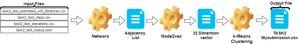
csv_writer . writerows ( random_data )任务2中的步骤可以总结如下:
Node2vec对邻接列表进行矢量列表。TASK2-Mysubmission.csv )是根据ID的轨迹准备的。这些步骤在下图中说明。
我们使用Python 3.6.5创建应用程序文件。我们包括了一些其他模块,这些模块未包含在比赛开始时给出的示例文件中。这些模块可以列为:
| molules | 任务 |
|---|---|
| Scikit-Learn | 机器学习和数据准备 |
| node2vec | 网络的可扩展功能学习 |
| numpy | 数学操作 |
我们从安装这些模块作为第一步。
 ## 2.1 Installing modules
!p ip install node2vec
!p ip install scikit - learn
!p ip install numpy 在此步骤中,我们修复了相关的随机种子以获得可重复的结果。这样,我们提供了一个确定性的路径,在每次运行中都会获得相同的结果。但是,根据我们的观察,在不同计算机上获得的结果可能略有不同(±1%)
 ## 2.2  Setting Random Seeds
seed_value = 0
import os
os . environ [ 'PYTHONHASHSEED' ] = str ( seed_value )
import random
random . seed ( seed_value )
import numpy as np
np . random . seed ( seed_value )在本节中,加载了用于测试数据的文件。
wifi变量从task2_test_estimated_wifi_distances.csv中获取ID和权重。steps变量从文件task2_test_steps.csv中获取ID和权重。elevs变量从文件task2_test_elevations.csv中获取ID。fp_lookup变量从task2_test_lookup.json文件中获取ID和轨迹。我们不希望使用Task1中获得的模型重新计算WiFi给出的估计距离的方法,因为我们从该过程中获得的结果没有显着差异。这就是为什么我们没有在最终工作中使用task2_test_fingerprints.json文件的原因。
 ## 2.3 Loading the data
import os
import json
import csv
import networkx as nx
from tqdm import tqdm

path_to_data = "task2_for_participants/test"

with open ( os . path . join ( path_to_data , "task2_test_estimated_wifi_distances.csv" )) as f :
    wifi = []
    reader = csv . DictReader ( f )
    for line in tqdm ( reader ):
        wifi . append ([ line [ 'id1' ], line [ 'id2' ], float ( line [ 'estimated_distance' ])])

with open ( os . path . join ( path_to_data , "task2_test_elevations.csv" )) as f :
    elevs = []
    reader = csv . DictReader ( f )
    for line in tqdm ( reader ):
        elevs . append ([ line [ 'id1' ], line [ 'id2' ]])

with open ( os . path . join ( path_to_data , "task2_test_steps.csv" )) as f :
    steps = []
    reader = csv . DictReader ( f )
    for line in tqdm ( reader ):
        steps . append ([ line [ 'id1' ], line [ 'id2' ], float ( line [ 'displacement' ])])

fp_lookup_path = os . path . join ( path_to_data , "task2_test_lookup.json" )

with open ( fp_lookup_path ) as f :
    fp_lookup = json . load ( f )
3773297it [00:19, 191689.25it/s]
2767it [00:00, 52461.27it/s]
139537it [00:00, 180082.01it/s]
创建轨迹图时,我们将平均距离作为权重。我们为任务2( Task2-IPS-Challenge-2021.ipynb )提供了此过程的示例。 We saved the resulting graph ( B ) as an adjacency list in the directory (as my.adjlist ).
 ## 2.3 Generating the Trajectory  graph.
B = nx . Graph ()

# Get all the trajectory ids from the lookup
valid_nodes = set ( fp_lookup . values ())

for node in valid_nodes :
    B . add_node ( node )

# Either add an edge or append the distance to the edge data
for id1 , id2 , dist in tqdm ( wifi ):
    if not B . has_edge ( fp_lookup [ str ( id1 )], fp_lookup [ str ( id2 )]):

        B . add_edge ( fp_lookup [ str ( id1 )],
                   fp_lookup [ str ( id2 )],
                   ty = "w" , weight = [ dist ])
    else :
        B [ fp_lookup [ str ( id1 )]][ fp_lookup [ str ( id2 )]][ 'weight' ]. append ( dist )

# Compute the mean edge weight
for edge in B . edges ( data = True ):
    B [ edge [ 0 ]][ edge [ 1 ]][ 'weight' ] = sum ( B [ edge [ 0 ]][ edge [ 1 ]][ 'weight' ]) / len ( B [ edge [ 0 ]][ edge [ 1 ]][ 'weight' ])

# If you have made a wifi connection between trajectories with an elev, delete the edge
for id1 , id2 in tqdm ( elevs ):
    if B . has_edge ( fp_lookup [ str ( id1 )], fp_lookup [ str ( id2 )]):
        B . remove_edge ( fp_lookup [ str ( id1 )],
                      fp_lookup [ str ( id2 )])

nx . write_adjlist ( B , "my.adjlist" )
100%|████████████████████████████████████████████████████████████████████| 3773297/3773297 [00:27<00:00, 135453.95it/s]
100%|██████████████████████████████████████████████████████████████████████████████████████| 2767/2767 [00:00<?, ?it/s]
Before giving the adjacency list as input to the machine learning algorithms, we convert the nodes to vector.在我们的工作中,我们将Node2Vec用作嵌入Grover&Leskovec在2016年提出的算法方法的图表[3]。 Node2Vec是一种半监督算法,用于网络中的节点的特征学习。 Node2Vec是基于跳过的技术创建的,该技术是一种NLP方法,该方法是出于分布结构概念的动机。根据想法,如果在相似上下文中使用的不同单词可能具有相似的含义,并且它们之间存在明显的关系。 Skip-gram技术使用中心词(输入)来预测邻居(输出),而基于给定的窗口大小(中心之后的项目的连续序列)计算周围环境的概率,换句话说。与NLP方法不同,Node2Vec系统不是带有线性结构的单词,而是具有分布式图形结构的节点和边缘。这种多维结构使嵌入式嵌入式复杂且计算昂贵,但是Node2Vec使用负抽样来优化随机梯度下降(SGD)来处理它。除此之外,随机步行方法还用于检测非线性结构中源节点相邻节点的样本。
在我们的研究中,我们首先通过从给定两个节点的给定距离(权重)的node2VEC建模低维空间中节点关系的矢量表示。然后,我们使用了带有节点向量的Node2Vec(图嵌入)的输出来馈送传统的K-均值聚类算法。
The parameters we use in Nod2vec can be listed as follows:
| 超参数 | 价值 |
|---|---|
| 方面 | 32 |
| walk_length | 15 |
| num_walks | 100 |
| 工人 | 1 |
| 种子 | 0 |
| 窗户 | 10 |
| min_count | 1 |
| batch_words | 4 |
Node2VEC模型将邻接列表作为输入列表,并输出32尺寸的向量。 In this part, the node.py file is created and run in the Jupyter Notebook .有两个原因是,最好在jupyter笔记本电脑单元格中运行外部而不是在外部运行。
Node2vec是一种非常昂贵的方法,如果在Jupyter Notebook中运行,则可能会出现RAM溢出错误。在外部创建和运行Node2vec模型避免了此错误。下面的单元格创建了名为node.py的文件。该文件创建Node2Vec模型。该模型将邻接列表( my.adjlist )作为输入,并创建一个32维向量文件作为输出( vectors.emb )。
重要的!下面的代码应在Linux发行版中运行(在Google Colab和Ubuntu中进行了测试)。
 # 2.4 Converting nodes to vectors
# A folder named tmp is created. This folder is essential for the node2vec model to use less RAM.
try :
    if not os . path . exists ( "tmp" ):
        os . makedirs ( "tmp" )
except OSError :
    print ( "The folder could not be created! n Please manually create the " tmp " folder in the directory" )


node = """

# importing related modules

from node2vec import Node2Vec
import networkx as nx

#importing  adjacency list file as B
B = nx.read_adjlist("my.adjlist")

seed_value=0


# Specifying the input and hyperparameters of the node2vec model
node2vec = Node2Vec(B, dimensions=32, walk_length=15, num_walks=100, workers=1,seed=seed_value,temp_folder = './tmp')

#Assigning/specifying random seeds

import os
os.environ['PYTHONHASHSEED']=str(seed_value)

import random
random.seed(seed_value)

import numpy as np
np.random.seed(seed_value)


# creation of the model

model = node2vec.fit(window=10, min_count=1, batch_words=4,seed=seed_value)


# saving the output vector

model.wv.save_word2vec_format("vectors.emb")

# save the model
model.save("vectorMODEL")

"""
f = open ( "node.py" , "w" )
f . write ( node )
f . close ()


! PYTHONHASHSEED = 0 python3 node . py 创建向量文件后,我们读取此文件( vectors.emb )。该文件由33列组成。第一列是节点号(ID),保留为矢量值。通过按第一列对整个文件进行排序,我们将节点返回其原始顺序。然后,我们删除此ID列,我们将不再使用。因此,我们给出数据的最终形状。我们的数据已准备好用于机器学习应用程序。
 # 2.4 Reshaping data
vec = np . loadtxt ( "vectors.emb" , skiprows = 1 )
print ( "shape of vector file: " , vec . shape )
print ( vec )
vec = vec [ vec [:, 0 ]. argsort ()];
vec = vec [ 0 : vec . shape [ 0 ], 1 : vec . shape [ 1 ]]
shape of vector file: (11162, 33)
[[ 9.1200000e+03 3.9031842e-01 -4.7147268e-01 ... -5.7490986e-02
1.3059708e-01 -5.4280665e-02]
[ 6.5320000e+03 -3.5591956e-02 -9.8558587e-01 ... -2.7217887e-02
5.6435770e-01 -5.7787680e-01]
[ 5.6580000e+03 3.5879680e-01 -4.7564098e-01 ... -9.7607370e-02
1.5506668e-01 1.1333219e-01]
...
[ 2.7950000e+03 1.1724627e-02 1.0272172e-02 ... -4.5596390e-04
-1.1507459e-02 -7.6738600e-04]
[ 4.3380000e+03 1.2865483e-02 1.2103912e-02 ... 1.6619096e-03
1.3672550e-02 1.4605848e-02]
[ 1.1770000e+03 -1.3707868e-03 1.5238028e-02 ... -5.9994194e-04
-1.2986251e-02 1.3706315e-03]]
Task-2是一个聚类问题。我们需要确定解决此问题的前提是我们应该分为多少个集群。为此,我们尝试了不同的集群数字,并比较了我们获得的分数。下图显示了簇数和获得的分数的比较。 As can be seen from this graph, the number of clusters increased continuously between 5 and 21, with some exception fluctuations, and stabilized after 21. For this reason, we focused on the number of clusters between 21 and 23 in our study.
 # 2.5 Determine the number of clusters
import numpy as np
import matplotlib . pyplot as plt
import seaborn as sns
import matplotlib
% matplotlib inline
sns . set_style ( "whitegrid" )
agglom = [ 24.69 , 28.14 , 28.14 , 28.14 , 30 , 33.33 , 40.88 , 38.70 , 40 , 40 , 40 , 29.12 , 45.85 , 45.85 , 48.00 , 50.17 , 57.83 , 57.83 , 57.83 ]
plt . figure ( figsize = ( 10 , 5 ))
plt . plot ( range ( 5 , 24 ), agglom )
matplotlib . pyplot . xticks ( range ( 5 , 24 ))
plt . title ( 'Number of clusters and performance relationship' )
plt . xlabel ( 'Number of clusters' )
plt . ylabel ( 'Score' )
plt . show ()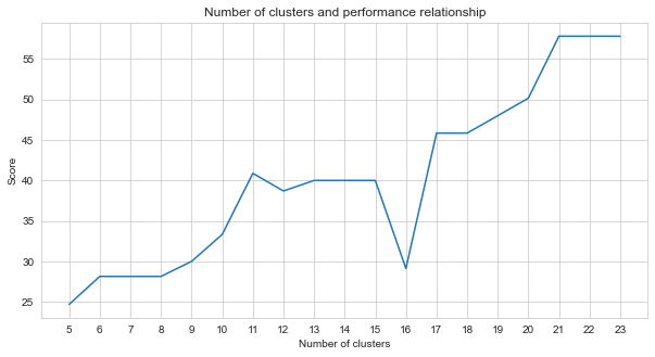
Among the unsupervised machine learning methods we tried (such as K-means, Agglomerative Clustering, Affinity Propagation, Mean Shift, Spectral clustering, DBSCAN, OPTICS, BIRCH, Mini-Batch K-Means), we achieved the best results using k-Means有23个集群。
K均值是一种聚类算法,是基本的,传统的无监督机器学习技术之一,它可以使用未标记的数据进行假设,以查找元素或自然组(群集)。集群是将共享特定相似之处分组在一起的一组点(我们的数据中的节点)。 K均值需要质心的目标数,这是指应将数据分为多少组。算法从随机分配的质心组开始,然后继续迭代以找到其最佳位置。该算法使用群集将点的正方形总和分配给指定的质心,这是继续更新和重新定位[4]。在我们的示例中,质心的数量反映了地板的数量。应该注意的是,这不会提供有关地板顺序的信息。
下面,已经为23个集群提供了K-均值应用程序。
 # 2.5  Best result
from sklearn import cluster
import time

ML_results = []
k_clusters = 23
algorithms = {}
algorithms [ 'KMeans' ] = cluster . KMeans ( n_clusters = k_clusters , random_state = 10 )
second = time . time ()
for model in algorithms . values ():
    model . fit ( vec )
    ML_results = list ( model . labels_ )
    print ( model , time . time () - second )
KMeans(n_clusters=23, random_state=10) 1.082334280014038
The output of the machine learning algorithm determines which cluster the fingerprints belong to.但是,我们需要的是群集轨迹。 Therefore, these fingerprints are converted to their trajectory counterparts using the fp_lookup variable.该输出被处理到TASK2-Mysubmission.csv文件中。
 ## 2.6 Submission
result = {}
for ii , i in enumerate ( set ( fp_lookup . values ())):
    result [ i ] = ML_results [ ii ]


ters = {}
for i in result :
    if result [ i ] not in ters :
        ters [ result [ i ]] = []
        ters [ result [ i ]]. append ( i )
    else :
        ters [ result [ i ]]. append ( i )


final_results = []
for i in ters :
    final_results . append ( ters [ i ])


name = "TASK2-Mysubmission.csv"
with open ( name , "w" , newline = '' ) as f :
    csv_writer = csv . writer ( f )
    csv_writer . writerows ( final_results )
print ( name , "file is ready!" )
TASK2-Mysubmission.csv file is ready!
[1] P. Virtanen和Scipy 1.0贡献者。 Scipy 1.0:Python中科学计算的基本算法。 Nature Methods, 17:261--272, 2020.
[2] A. Geron,Scikit-Learn,Keras和TensorFlow的动手机器学习:构建智能系统的概念,工具和技术。 O'Reilly Media,2019年
[3] A. Grover,J。Leskovec。 ACM SIGKDD国际知识发现与数据挖掘会议(KDD),2016年。
[4] Jin X.,Han J.(2011)K-均值聚类。 In: Sammut C., Webb GI (eds) Encyclopedia of Machine Learning.马萨诸塞州波士顿的施普林格。 https://doi.org/10.1007/978-0-387-30164-8_425


