smard power forecasting
1.0.0
該儲存庫用於預測德國的電力消耗。
基於並受到以下啟發:
資料來源:SMARD
將所有下載的檔案放入:
/example/dataset # there is already used dataset included if you pull, but you could update
檢查 Forecast.Rmd 檔案以了解如何在更新版本的 SMARD-Data 上執行此程式碼。
使用的函式庫:
 # Probably needed
# Load Packages
# library(fhswf)
# library(tsibbledata)
# library(broom)
# library(readr)
# library(datasets)
# library(timeDate)
# library(qlcal)
# library(corrplot)
# library(mgcv)
# library(MEFM)
# library(TTR)

packages <- c(
  "devtools",
  "ggplot2",
  "dplyr",
  "tsibble",
  "fable",
  "fabletools",
  "feasts",
  "distributional",
  "lubridate",
  "tidyr",
  "forecast",
  "zoo",
  "scales",
  "fable.prophet"
)
install.packages(packages)


library(devtools)
library(ggplot2)
library(dplyr)
library(tsibble)
library(fable)
library(fabletools)
library(feasts)
library(distributional)
library(lubridate)
library(tidyr)
library(forecast)
library(zoo)
library(scales)
library(fable.prophet)
嘗試在 example/ 資料夾中開始工作。
 # Define datapaths
power_consum_path <- "dataset\stunde_2015_2024\Realisierter_Stromverbrauch_201501010000_202407090000_Stunde.csv"
power_consum_smard_prediction_path <- "dataset\propgnose_vom_smard\Prognostizierter_Stromverbrauch_202401010000_202407090000_Stunde.csv"

# Load Smard Prediction
power_consum_smard_prediction_loaded <- load_power_consum(path=power_consum_smard_prediction_path)
raw_smard_pred <- power_consum_smard_prediction_loaded$raw_data
cleaned_smard_pred <- power_consum_smard_prediction_loaded$cleaned_data

cleaned_smard_pred <- cleaned_smard_pred |>
  mutate(.model = "SMARD")
names(cleaned_smard_pred)[names(cleaned_smard_pred) == "PowerConsum"] <- ".mean"

# Load PowerConsum Data
power_consum_loaded <- load_power_consum(path=power_consum_path)
raw_power_consum <- power_consum_loaded$raw_data
cleaned_power_consum <- power_consum_loaded$cleaned_data

# Generate more features
cleaned_power_consum$localName[is.na(cleaned_power_consum$localName)] = "Working-Day"
cleaned_power_consum$MeanLastWeek <- rollapply(cleaned_power_consum$PowerConsum, width = 24*8, FUN = function(x) mean(x[1:(24*8-25)]), align = "right", fill = NA)
cleaned_power_consum$MeanLastTwoDays <- rollapply(cleaned_power_consum$PowerConsum, width = 24*3, FUN = function(x) mean(x[1:(24*3-25)]), align = "right", fill = NA)
cleaned_power_consum$MaxLastOneDay <- rollapply(cleaned_power_consum$PowerConsum, width = 24*2, FUN = function(x) max(x[1:(24*2-25)]), align = "right", fill = NA)
cleaned_power_consum$MinLastOneDay <- rollapply(cleaned_power_consum$PowerConsum, width = 24*2, FUN = function(x) min(x[1:(24*2-25)]), align = "right", fill = NA)
以下功能是從資料集和假日 API 產生的:
| 指數 | 列名 | 描述 |
|---|---|---|
| 1 | 日期從 | 用於驗證 DateIndex(類似,但原始) |
| 2 | 耗電量 | 功耗(MW) |
| 3 | 日期索引 | 時間戳記 (yyyy-mm-dd hh:mm:ss) |
| 4 | 工作日 | Mo、Di、Mi、Do、Fr、Sa、So(德文工作日) |
| 5 | 日期 | 日期(年-月-日) |
| 6 | 年 | 年份 yyyy |
| 7 | 星期 | 週數 0-53 |
| 8 | 小時 | 小時數 0-24 |
| 9 | 月 | 月份號 1-12 |
| 10 | 本地名稱 | 時間戳記的假日名稱 |
| 11 | 工作日 | 1/0 如果是工作日(Werktag)則 1 |
| 12 | 莫 | 1/0 若星期一則 1 |
| 13 | 迪 | 1/0 如果星期二則 1 |
| 14 | 米 | 1/0 若星期三則 1 |
| 15 | 做 | 1/0 若星期四則 1 |
| 16 | Fr | 1/0 如果星期五則 1 |
| 17 號 | 薩 | 1/0 若星期六則 1 |
| 18 | 所以 | 1/0 如果週日則 1(如果使用週一至週六則不需要) |
| 19 | 假期 | 1/0 如果是假日則 1 |
| 20 | 平日假日週末 | 如果是假期、週末或工作日(對於地塊,是字元。) |
| 21 | 假期和工作日 | 1/0 若假期為工作日則 1 |
| 22 | 最後一天不是工作日 | 1/0 如果最後一天不是工作日則 1 |
| 23 | 最後一天不是工作日而現在是工作日 | 1/0 如果最後一天不是工作日而現在是工作日則 1 |
| 24 | 下一天不是工作日並且現在是工作日 | 1/0 如果第二天不是工作日而現在是工作日則 1 |
| 25 | 最後一天是假期而不是週末 | 1/0 如果最後一天是假日而不是週末,則 1 |
| 26 | 下一天是假日而不是週末 | 1/0 如果第二天是假日而不是週末,則 1 |
| 27 | 假期名稱 | 類似於 localName(假期名稱) |
| 28 | 年底 | 1/0 如果是年底(第 52 或 53 週) |
| 29 | 新年第一周 | 1/0 如果是年初(第一週) |
| 30 | 假期延長 | 1/0 滯後假期(第二天 6 小時) |
| 31 | 假期平滑 | 假期延長 + sin(2*pi(小時)+1)/24) |
| 32 | 平均上週 | 上週平均耗電量(班次:24*8-25) |
| 33 | 平均最後兩天 | 近兩天平均耗電量(班次:24*3-25) |
| 34 | 最大最後一天 | 最後一天的最大耗電量(班次:24*2-25) |
| 35 | 最短最後一天 | 最後一天的最小耗電量(班次:24*2-25) |
在這項研究中,有來自 SMARD 的 2015 - 2024 年德國電力消耗資料集。
圖 1 顯示了原始資料集,其中包含缺失值(紅色)、重複的時間戳記(深紅色)和隨時間變化的功耗(灰色)、每小時解析度。每年有一個缺失值和一個重複值,因此很容易清理資料集。總體而言,這是一個幾乎乾淨的集合。清理資料集後,可以對功耗進行合理的觀察:
有一種簡單的方法可以透過最後一次觀察來填補空白(這是可能的,因為解析度足夠大且只有很少的缺失值)。第一個值被保留以用於重複。
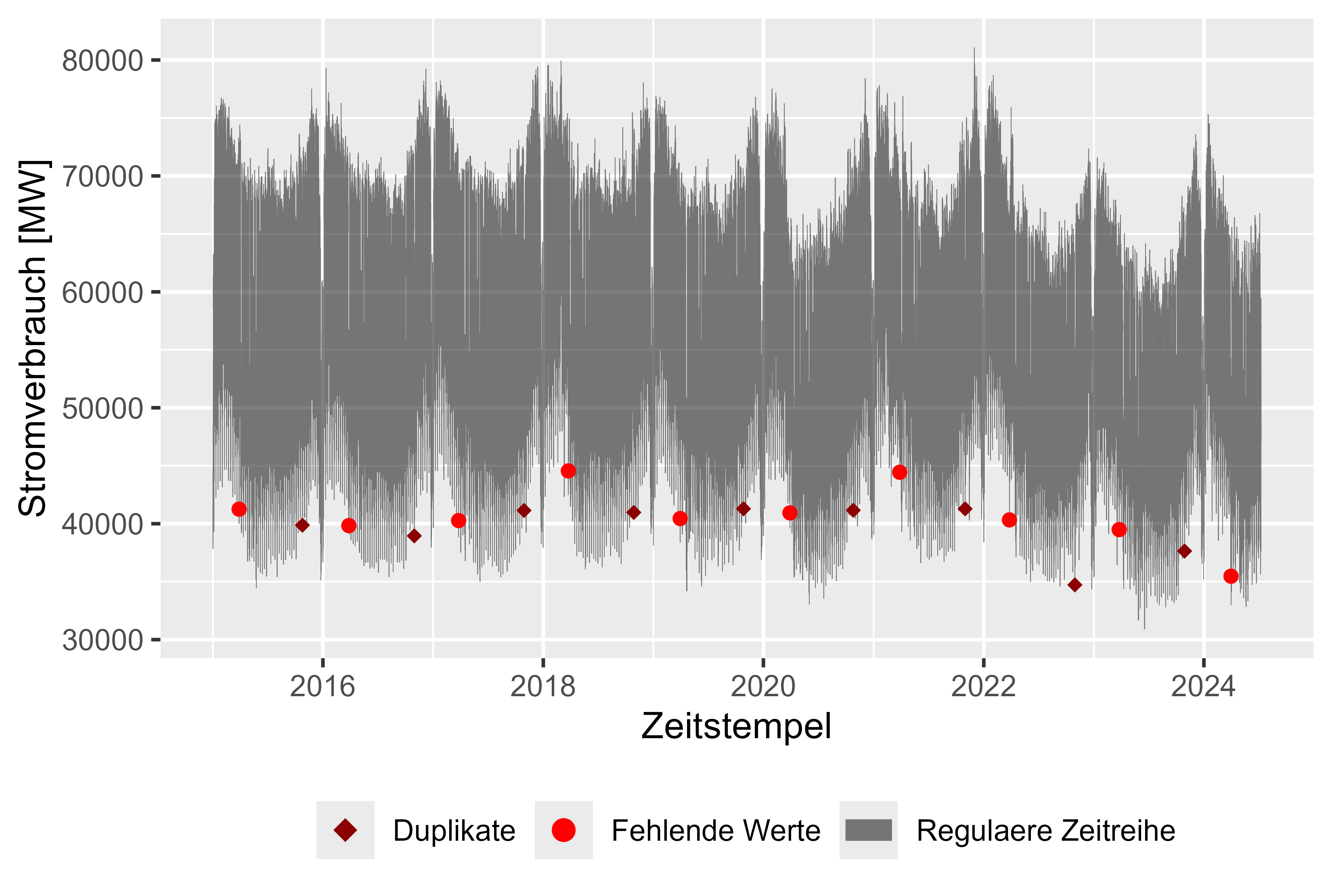 圖1 原始功耗
 local_name_colors <- c(
  "Christi Himmelfahrt" = palette()[2],
  "Erster Weihnachtstag" = palette()[2],
  "Karfreitag" = palette()[2],
  "Neujahr" = palette()[2],
  "Ostermontag" = palette()[2],
  "Pfingstmontag" = palette()[2],
  "Reformationstag" = palette()[2],
  "Tag der Arbeit" = palette()[2],
  "Tag der Deutschen Einheit" = palette()[2],
  "Zweiter Weihnachtstag" = palette()[2],
  "Regulärer Tag" = palette()[1]
)


week_colors <- c(
  "Mo" = palette()[1],
  "Di" = palette()[1],
  "Mi" = palette()[1],
  "Do" = palette()[1],
  "Fr" = palette()[1],
  "Sa" = palette()[2],
  "So" = palette()[2]
)

working_colors <- c("1" = "#2E9FDF", "0" = "#FC4E07")

whw_colors <- c(
  "FeiertagnKein Wochenende" = "black",
  "Kein FeiertagnKein Wochenende" = "red",
  "Kein FeiertagnWochenende" = "orange",
  "FeiertagnWochenende" = "blue"
)

p <- cleaned_power_consum |>
    gg_tsdisplay(PowerConsum, plot_type = "partial", lag = 100)

ggsave(
  "plots/power_consum_acf_pacf.png",
  plot = p,
  width = 5.5,
  height = 3.7,
  dpi = 600
)

plot_calculated_features(
  cleaned_power_consum = cleaned_power_consum,
  file_name = "plots/MinLastOneDay.png",
  x = "MinLastOneDay",
  y = "PowerConsum",
  x_label = "Minimaler Stromverbrauch vom letzten Tag [MW]",
  y_label = "Stromverbrauch [MW]"
)

plot_calculated_features(
  cleaned_power_consum = cleaned_power_consum,
  file_name = "plots/MaxLastOneDay.png",
  x = "MaxLastOneDay",
  y = "PowerConsum",
  x_label = "Maximaler Stromverbrauch vom letzten Tag [MW]",
  y_label = "Stromverbrauch [MW]"
)

plot_calculated_features(
  cleaned_power_consum = cleaned_power_consum,
  file_name = "plots/MeanLastWeek.png",
  x = "MeanLastWeek",
  y = "PowerConsum",
  x_label = "Durchschnittlicher Stromverbrauch der letzten 7 Tage [MW]",
  y_label = "Stromverbrauch [MW]"
)


plot_calculated_features(
  cleaned_power_consum = cleaned_power_consum,
  file_name = "plots/MeanLastTwoDays.png",
  x = "MeanLastTwoDays",
  y = "PowerConsum",
  x_label = "Durchschnittlicher Stromverbrauch der letzten 2 Tage [MW]",
  y_label = "Stromverbrauch [MW]"
)

plot_histogram_by_group(
  cleaned_power_consum,
  group_name = "WorkdayHolidayWeekend",
  file_name = "plots\workday_holiday_weekend_histogram.png",
  colors = whw_colors,
  x="PowerConsum",
  x_label = "Stromverbrauch [MW]",
  y_label = "Häufigkeit",
  name_0 = "Wochenende oder Feiertage",
  name_1 = "Werktag"
)


plot_histogram_by_group(
  cleaned_power_consum,
  group_name = "WorkDay",
  file_name = "plots\workday_histogram.png",
  colors = working_colors,
  x="PowerConsum",
  x_label = "Stromverbrauch [MW]",
  y_label = "Häufigkeit",
  name_0 = "Wochenende oder Feiertage",
  name_1 = "Werktag"
)

plot_histogram_by_group(
  cleaned_power_consum,
  group_name = "Holiday",
  file_name = "plots\holiday_histogram.png",
  colors = working_colors,
  x="PowerConsum",
  x_label = "Stromverbrauch [MW]",
  y_label = "Häufigkeit",
  name_0 = "Werktag oder Wochenende",
  name_1 = "Feiertag"
)

plot_histogram_by_group(
  cleaned_power_consum,
  group_name = "HolidayAndWorkDay",
  file_name = "plots\holiday_workday_histogram.png",
  colors = working_colors,
  x="PowerConsum",
  x_label = "Stromverbrauch [MW]",
  y_label = "Häufigkeit",
  name_0 = "Wochenende oder Werktag",
  name_1 = "Feiertag am Werktag"
)

plot_by_group(
  cleaned_power_consum,
  group_name = "HolidayName",
  file_name = "plots\holiday_boxplot.png",
  colors = local_name_colors,
  title = "Übersicht der einzelnen Feiertage",
  y="PowerConsum",
  y_label="Stromverbrauch [MW]",
  x_label="Jahre"
)

plot_by_group(
  cleaned_power_consum,
  group_name = "Weekday",
  file_name = "plots\weekday_boxplot.png",
  colors = week_colors,
  title = "Übersicht der einzelnen Wochentage",
  y = "PowerConsum",
  y_label="Stromverbrauch [MW]",
  x_label="Jahre"
)

plot_by_group(
  cleaned_power_consum,
  group_name = "WorkDay",
  file_name = "plots\workday_boxplot.png",
  colors = working_colors,
  title = "Übersicht, ob Feiertag (FALSE) oder Werktag (TRUE)",
  y = "PowerConsum",
  y_label="Stromverbrauch [MW]",
  x_label="Jahre"
)


plot_by_column(
  df = cleaned_power_consum,
  x = "Hour",
  y = "PowerConsum",
  x_label = "Stunden",
  y_label = "Stromverbrauch [MW]",
  file_name = "plots\hour_boxplot.png",
  title = "Übersicht der einzelnen Stunden"
)

plot_by_column(
  df = cleaned_power_consum,
  x = "Month",
  y = "PowerConsum",
  x_label = "Monate",
  y_label = "Stromverbrauch [MW]",
  file_name = "plots\month_boxplot.png",
  title = "Übersicht der einzelnen Monate"
)

plot_by_column(
  df = cleaned_power_consum,
  x = "Week",
  y = "PowerConsum",
  x_label = "Woche",
  y_label = "Stromverbrauch [MW]",
  file_name = "plots\week_boxplot.png",
  title = "Übersicht der einzelnen Wochen"
)

plot_by_column(
  df = cleaned_power_consum,
  x = "Year",
  y = "PowerConsum",
  x_label = "Jahr",
  y_label = "Stromverbrauch [MW]",
  file_name = "plots\year_boxplot.png",
  title = "Übersicht der einzelnen Jahre"
)

plot_year_month_week_day(
  df=cleaned_power_consum,
  date_column="DateIndex",
  y="PowerConsum",
  from_year=2015,
  to_year=2024,
  from_week=0,
  to_week=53,
  year_for_week=2018,
  from_day=1,
  to_day=30,
  month_for_day=4,
  year_for_day=2018,
  from_month=1,
  to_month=12,
  year_for_month=2018,
  holiday="Holiday",
  day_of_week = "Weekday"
)
以下部分將越來越詳細地介紹數據。我們將從年度代表開始。
圖 2 是 2015-2024 年的年度圖。這裡我們可以注意到,年初用電量增加,年底用電量減少(聖誕節、新年)。整體看起來像微笑形狀或蝴蝶結。
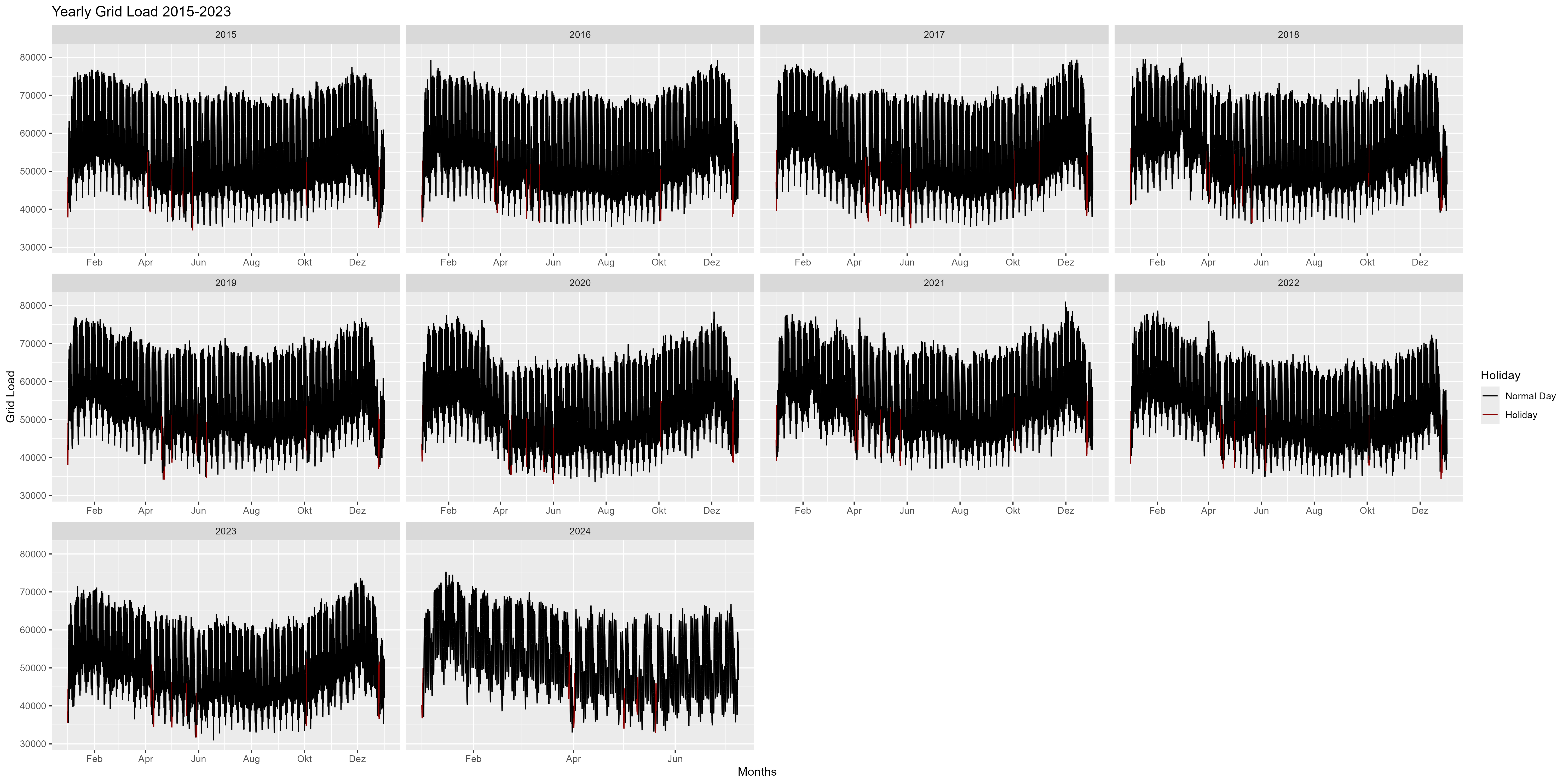 圖 2 每年的功耗
讓我們嘗試匯總所有年份並將它們分成幾週。圖 3 中的箱線圖結合了所有年份。我們可以更詳細地看到該模式。一年的開始和結束以紅色表示,並顯示出與常規「微笑形狀」相比有所減少。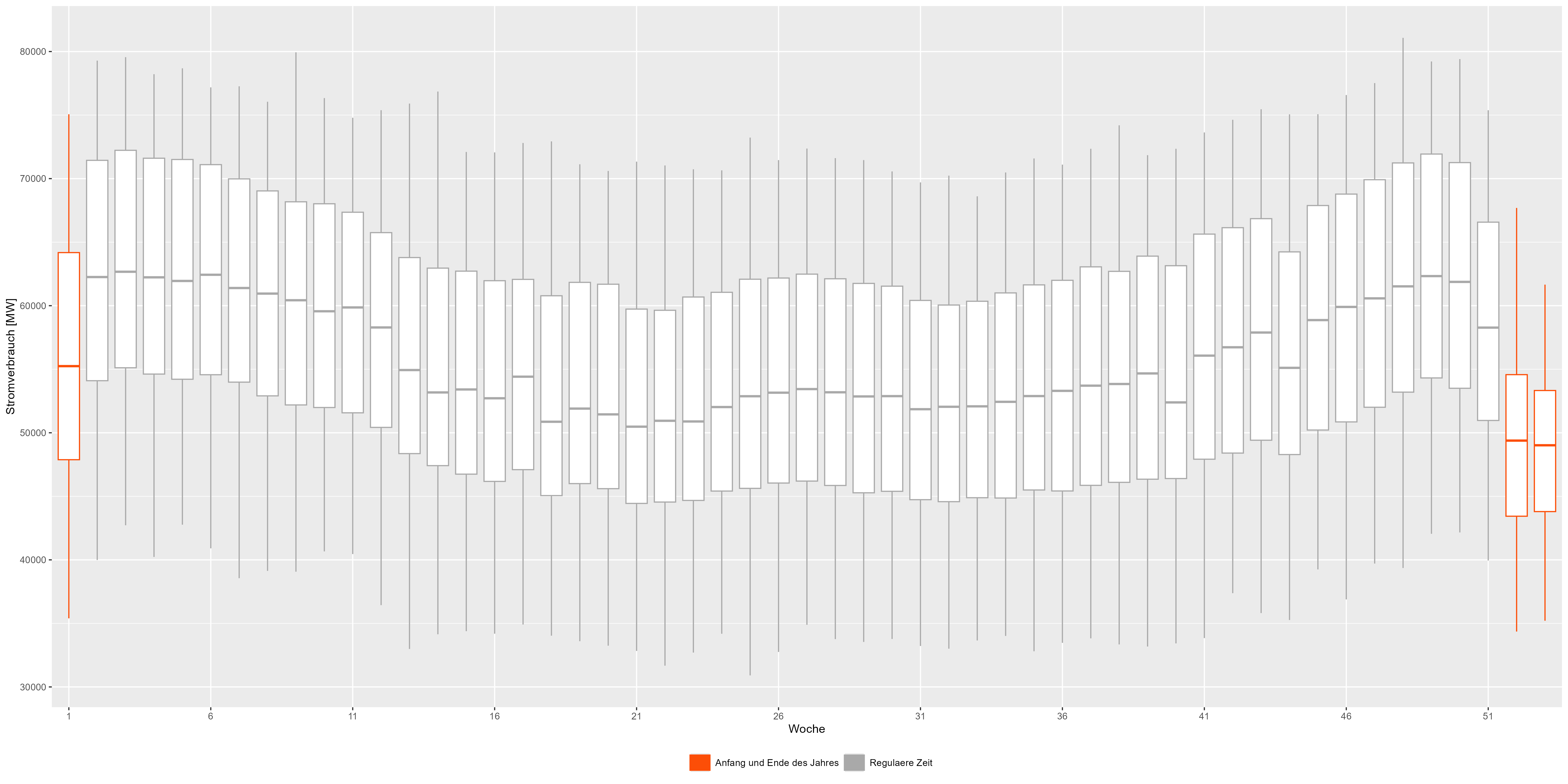 圖3 每周用電量彙總數據
讓我們更詳細地了解一下,例如 2018 年。圖4是2018年的月圖。 12月24日左右,用電量有所下降。這裡也值得注意的是週末和假日(紅色)。所有週末和所有假日都會減少。
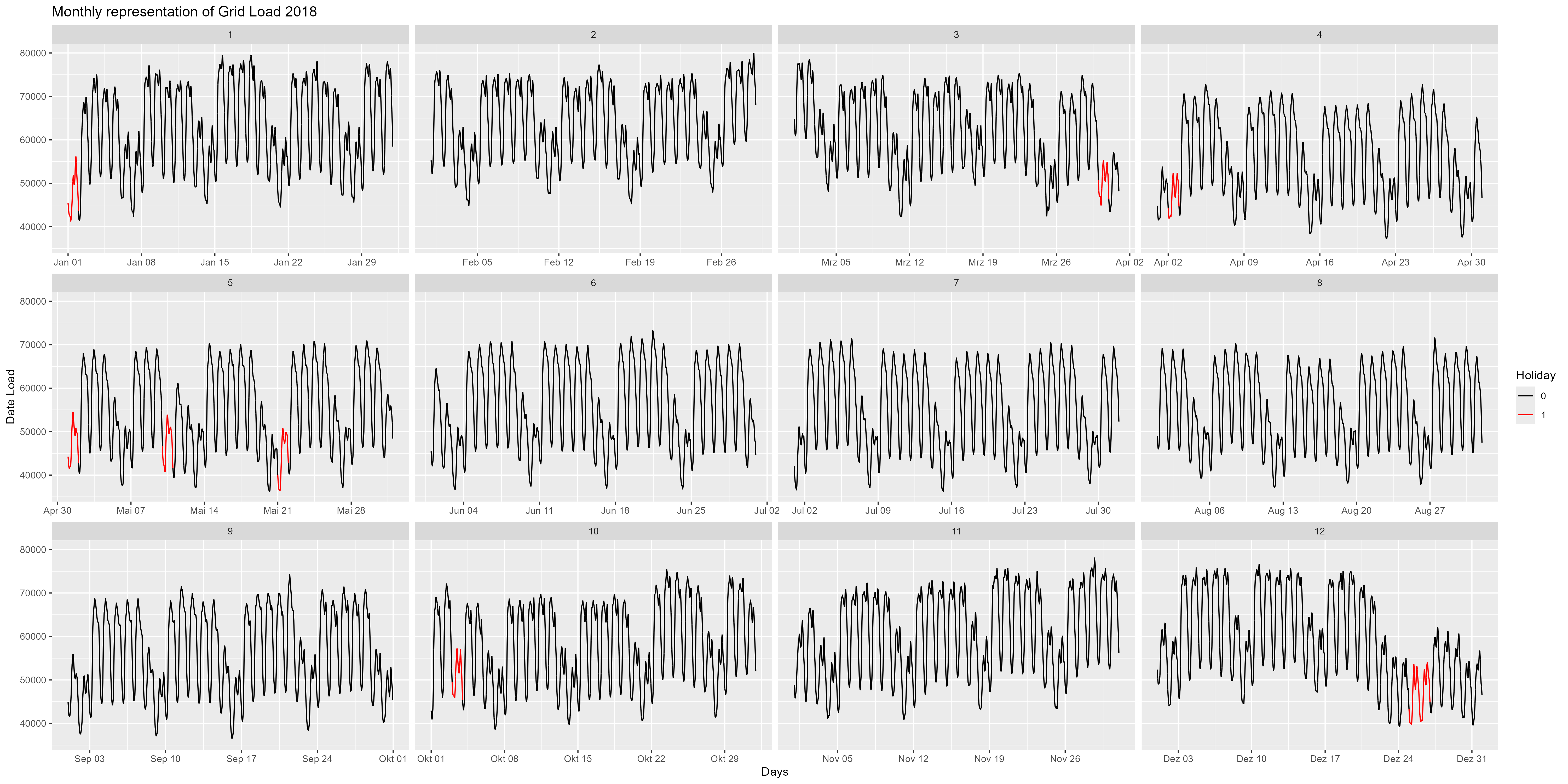 圖 4 每月的功耗,作為一個面向
我們可以更進一步查看數據的每小時表示。圖 5 顯示了每小時的聚合箱線圖。夜間(21:00-06:00)也減少,白天/工作時間(06:00-21:00)增加。也是需要包含在模型中的模式。
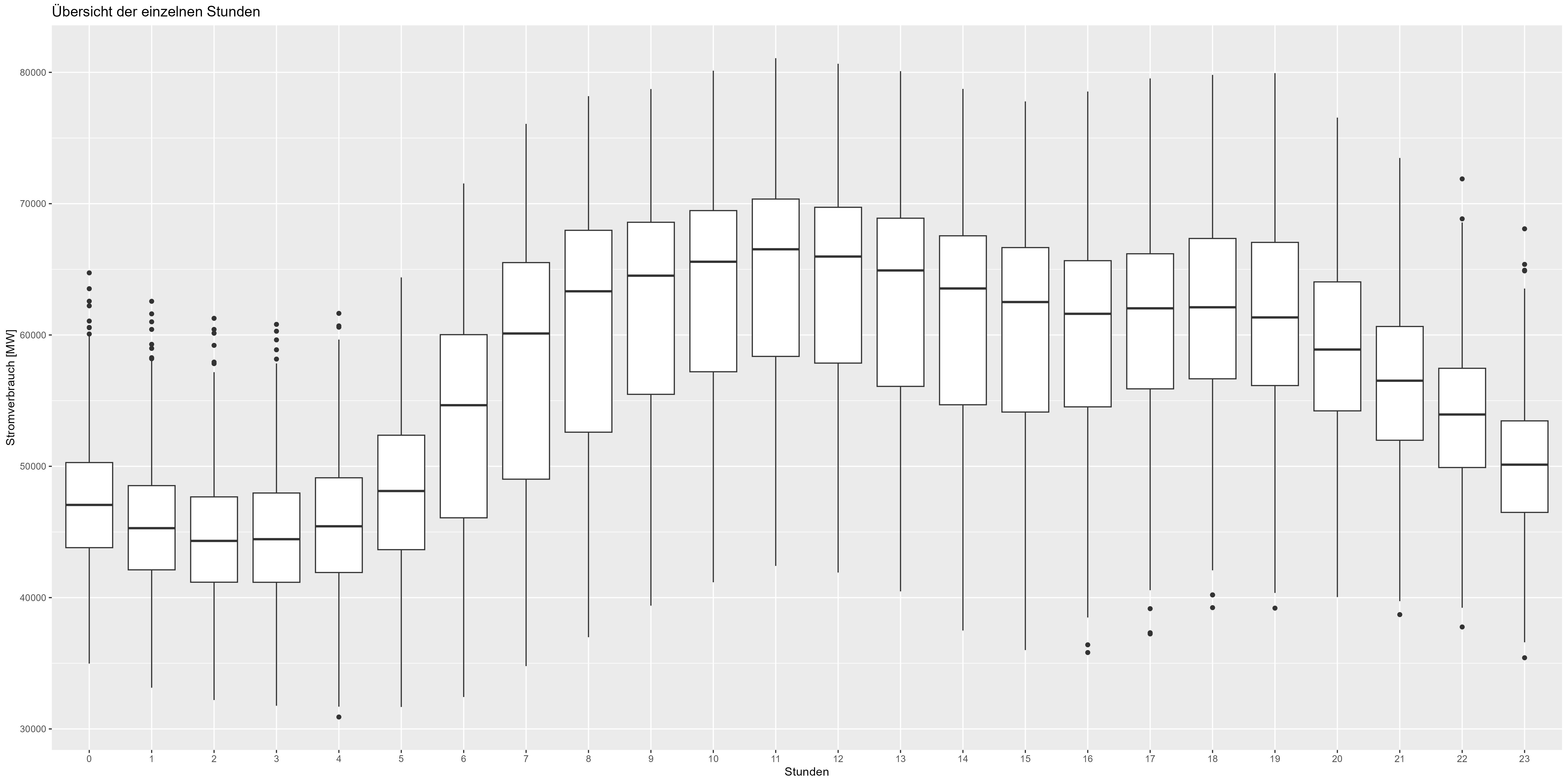 圖5 每小時用電量彙總數據
我們來談談工作日吧。正如所假設的,週末電力消耗會減少。 「Durchschnitt」是意思。圖 6 顯示了多年來所有的工作日(總結)。週末減少約 10,000 MW。
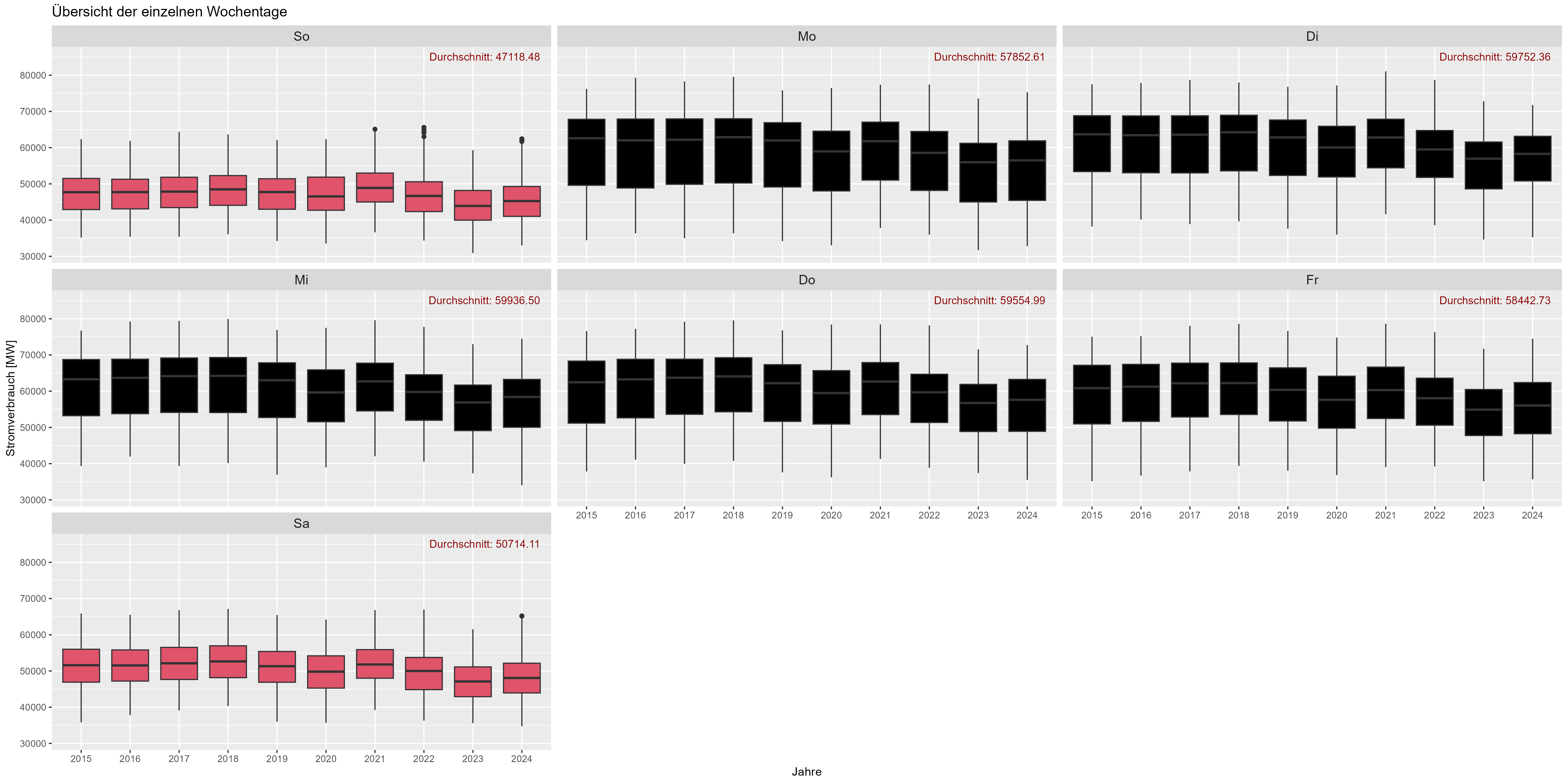 圖 6 功耗“週內效應”
圖8顯示了假期效果。 「Durchschnitt」是多年來的平均耗電量。與假日(紅色)相比,「工作日」(深灰色)的耗電量顯著增加。我們可以假設假期對於電力消耗來說就像週末一樣」。
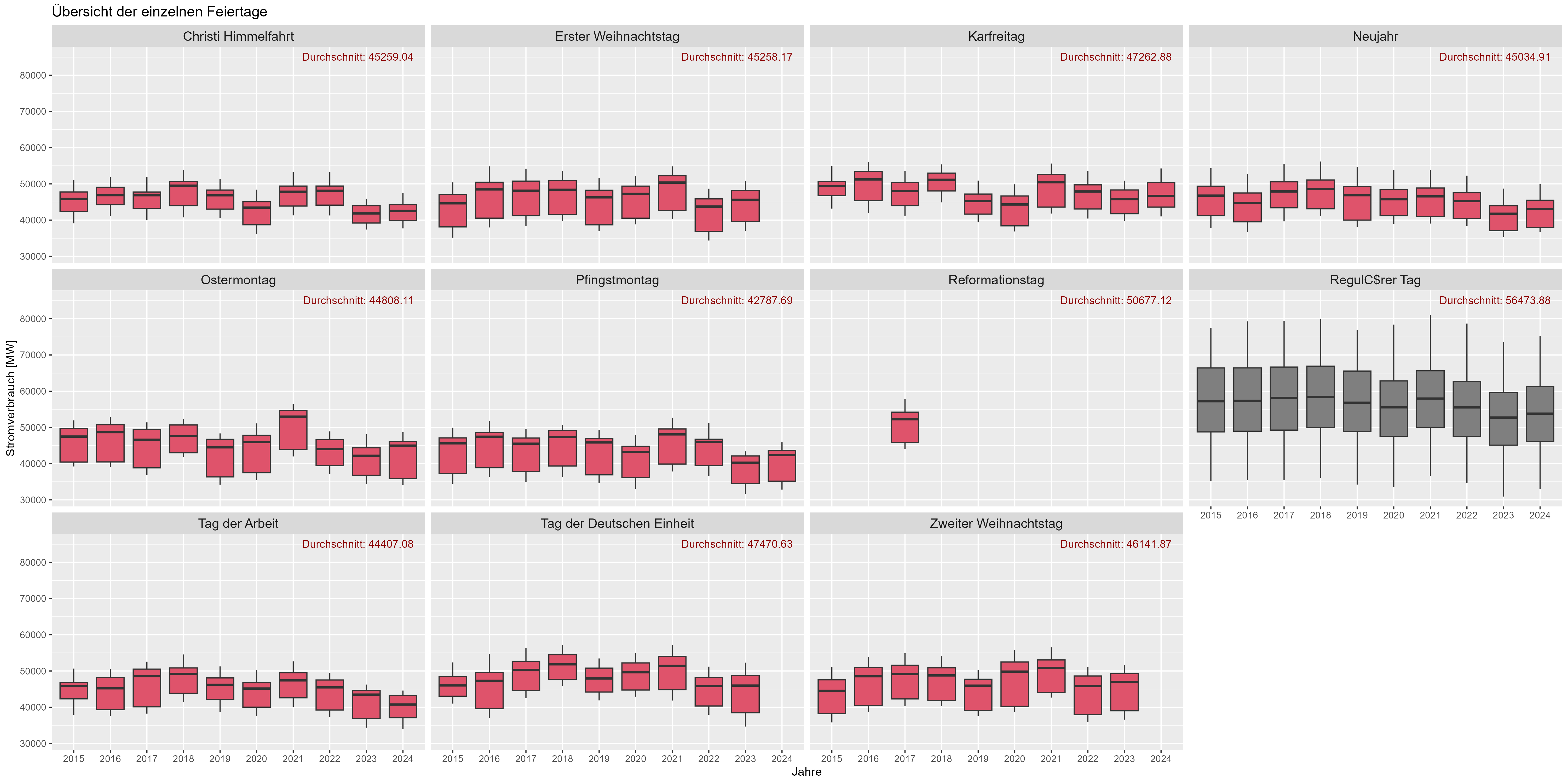 圖6 功耗“假期效應”
圖 7 代表不同日期的不同行為。有 4 類。 「Feiertag Kein Wochenende」的意思是這是一個假期,但不是週末。 「Feiertag Wochenende」的意思是這是一個假期和一個週末。 「Kein Feiertag Kein Wochenende」表示這是一個正常工作日,「Kein Feiertag Wochenende」表示這只是週末。我們可以觀察到假設的非正常工作日的類似分佈。
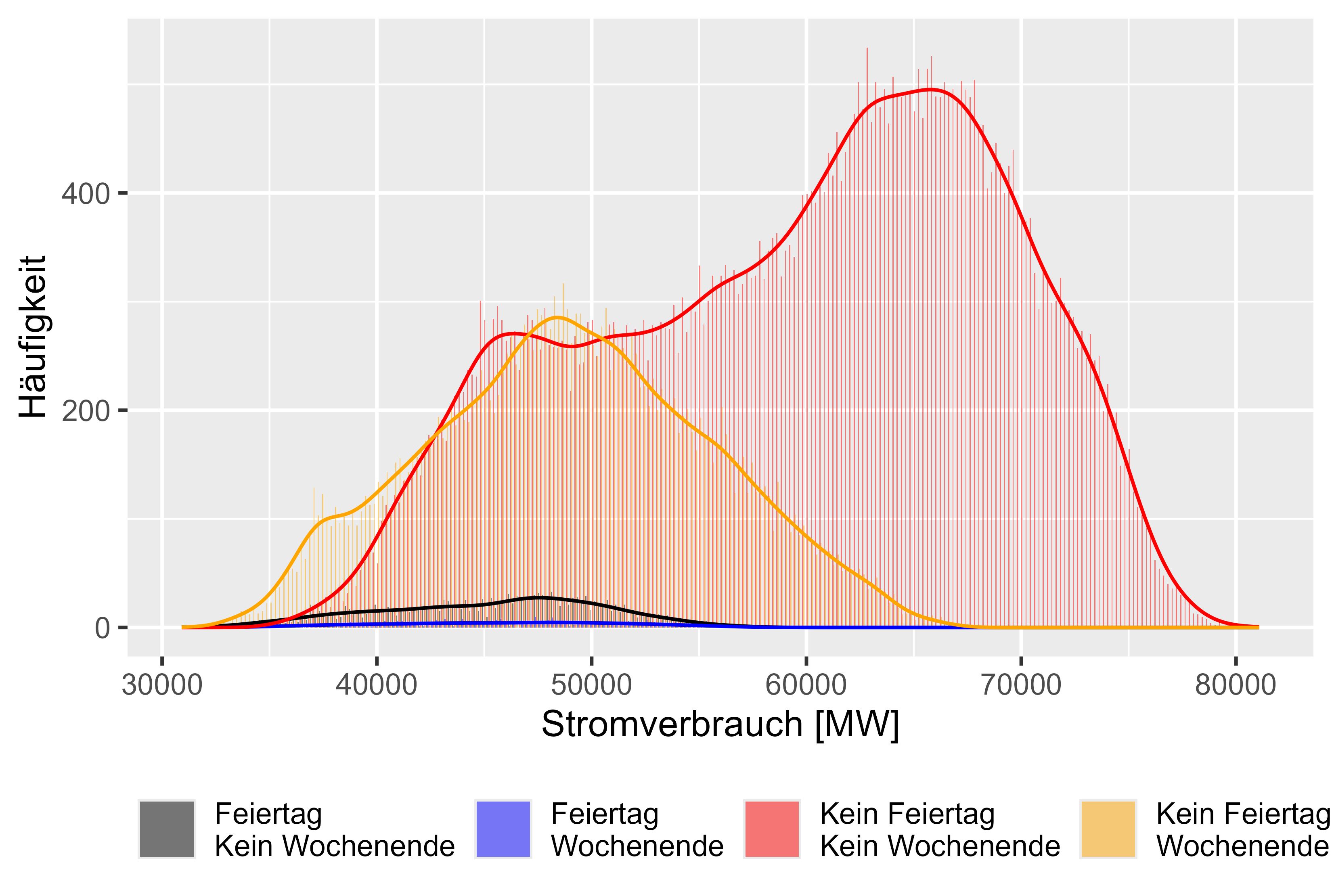 圖7 功耗「不同效果」比較
MeanLastTwoDays、MeanLastWeek、MaxLastOneDay 和 MinLastOneDay 等滯後值是產生的特徵。
與 DOI 中討論的類似:10.1109/TPWRS.2011.2162082 - 基於半參數加性模型的短期負載預測
圖 8-11(紅色不是工作日)表示相對於實際功耗的滯後值。
這個生成的特徵有輕微的相關性。
 # Check Correlation
cor <- cor(cleaned_power_consum[sapply(cleaned_power_consum, is.numeric)], method = c("pearson", "kendall", "spearman"), use = "complete.obs")
| 特徵 | 與功耗的相關性 |
|---|---|
| 假期平滑 | -0.556194 |
| 平均上週 | 0.389044 |
| 平均最後兩天 | 0.201253 |
| 最大最後一天 | 0.320193 |
| 最短最後一天 | 0.348583 |
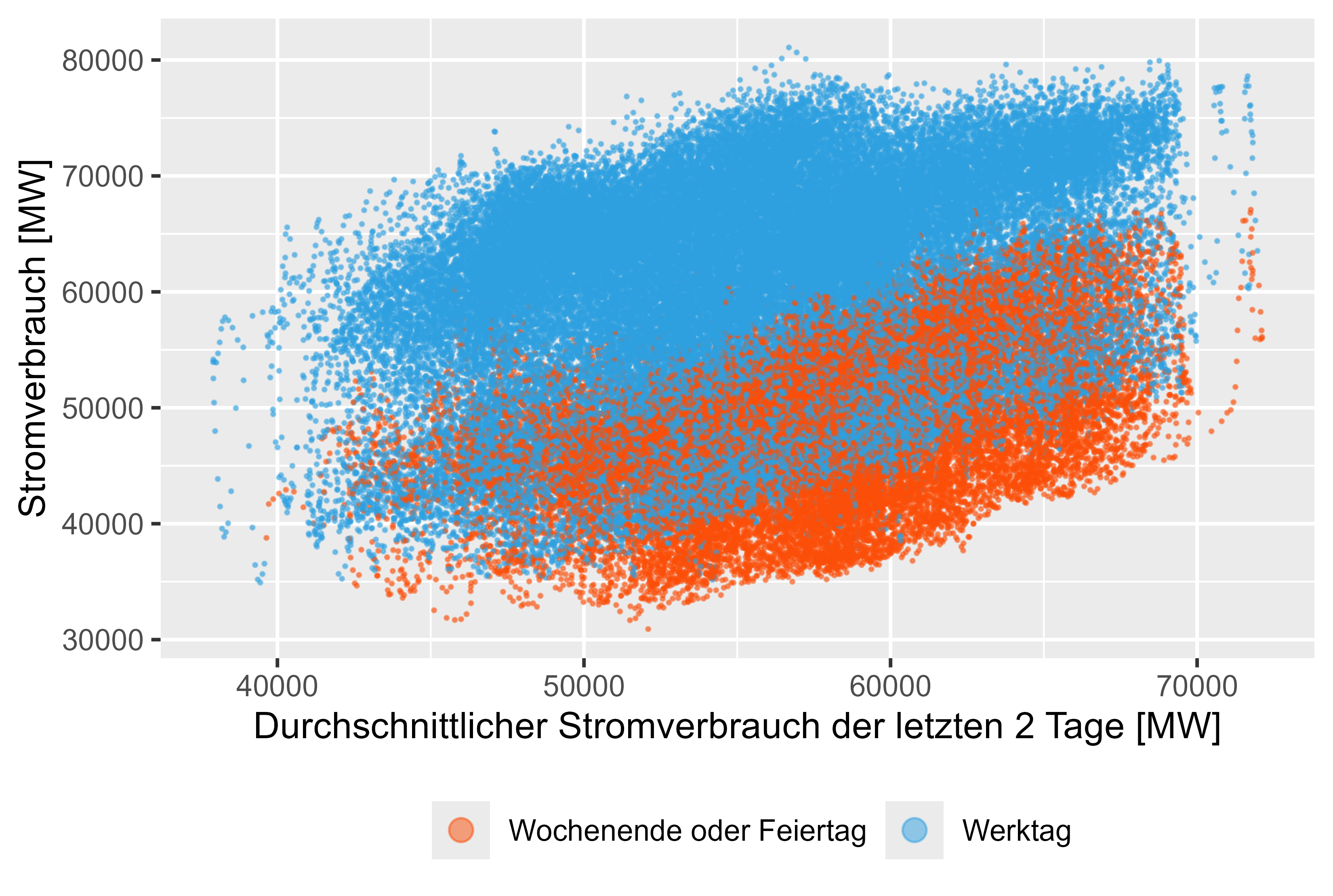 圖 8 耗電量 - MeanLastTwoDays
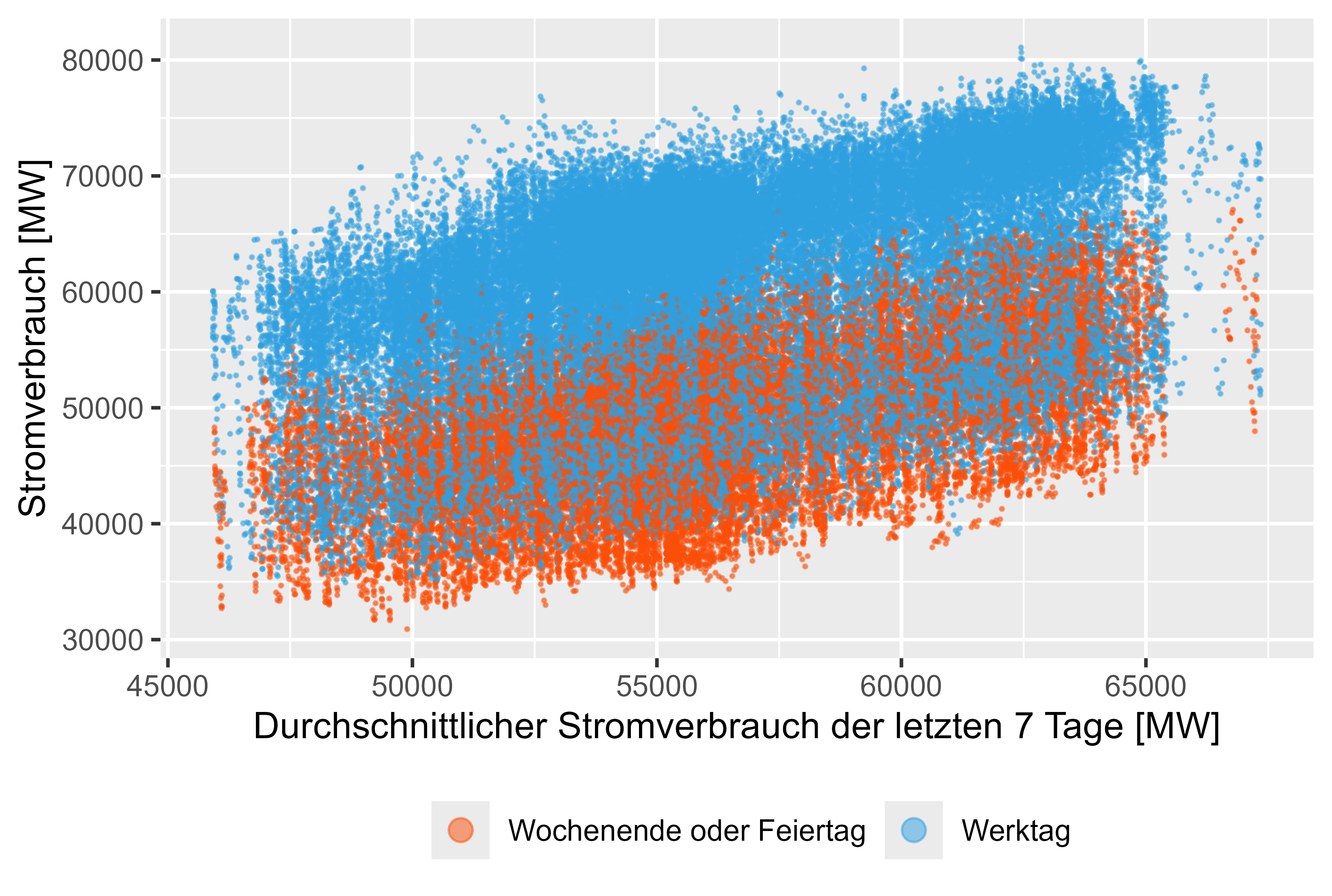 圖 9 耗電量 - MeanLastWeek
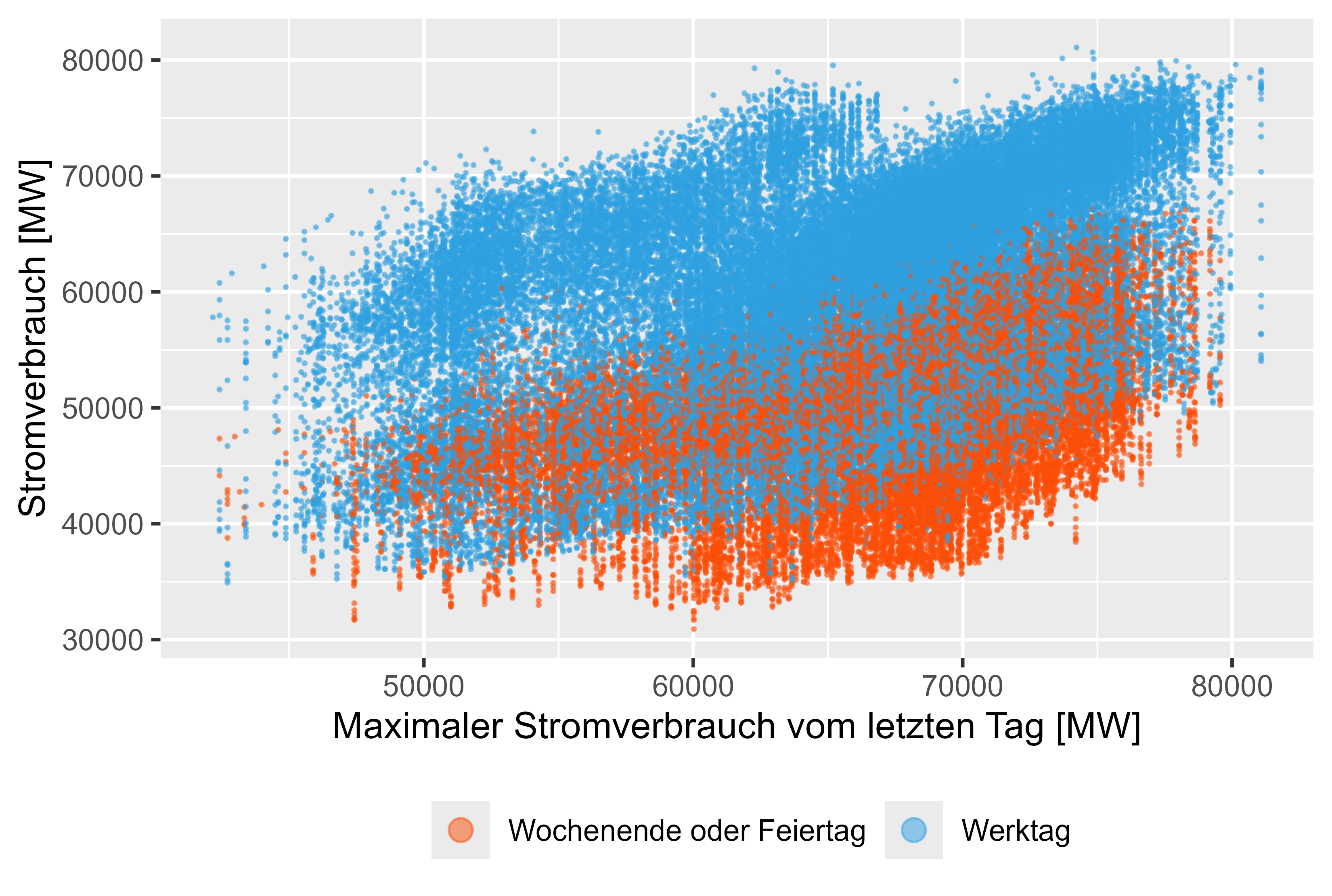 圖 10 耗電量 - MaxLastOneDay
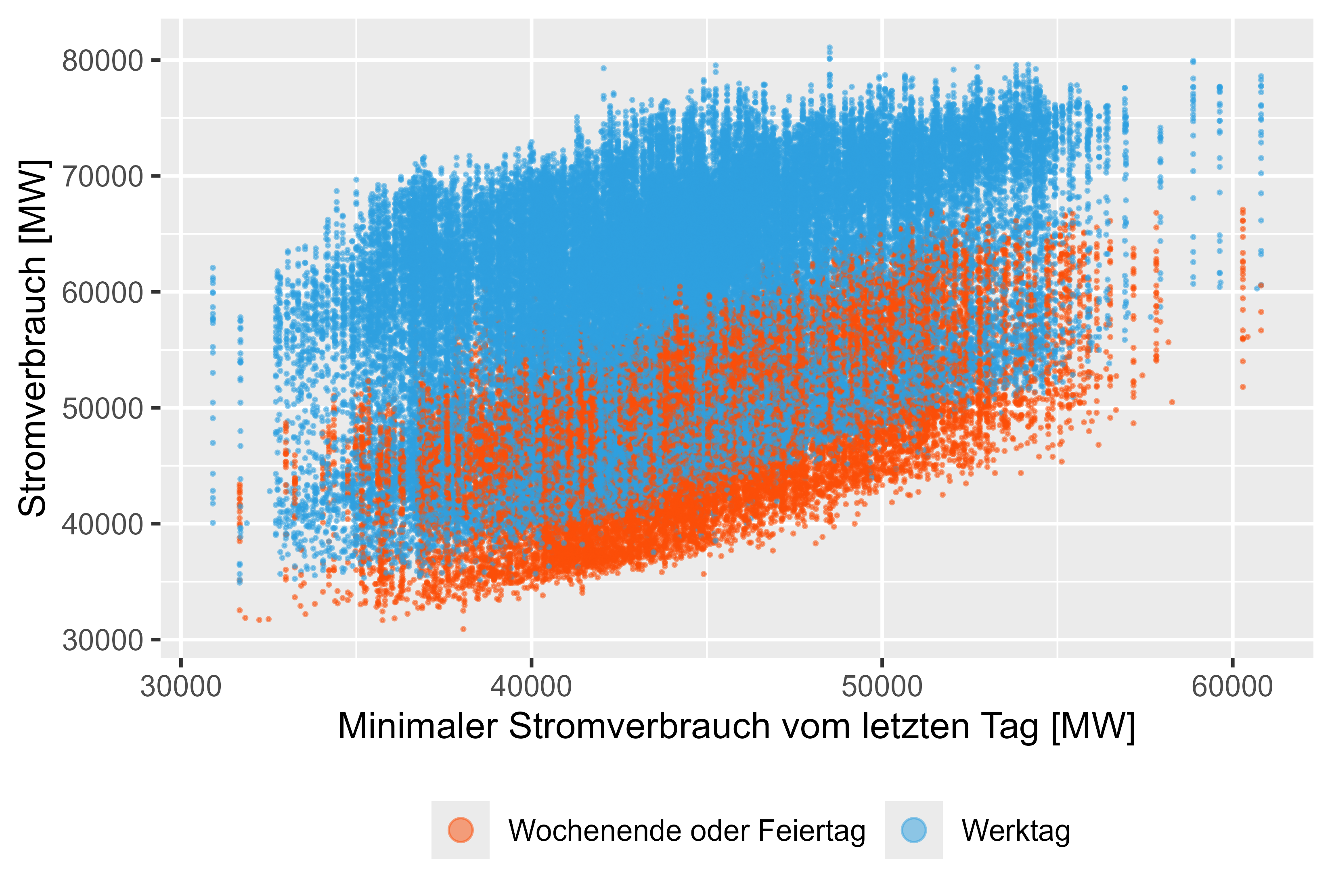 圖 11 功耗 - MinLastOneDay
存在複雜的季節性。對於每小時分辨率,有每年、每周和每日的季節性。這需要由模型追蹤。這裡的解決方案如預測:原理與實踐第 12.1 章複雜季節性中所述,使用傅立葉項透過 cos() 和 sin() 表示和組裝複雜季節性。
我們可以看一下 ACF 和 PACF 圖,幾乎沒有顯著的尖峰,但它只是 96 個滯後值的表示。如果我們採用一年約 9000 個滯後觀測值,就會出現複雜的季節性。這就是為什麼使用傅立葉項會比較容易。僅透過以下方式尋找 PDQ 和 pdq 組件也效果不佳
 ARIMA(...
stepwise=FALSE,
greedy=FALSE,
approx=FALSE)
本身。如果沒有傅立葉項,訓練時間也會急遽增加。
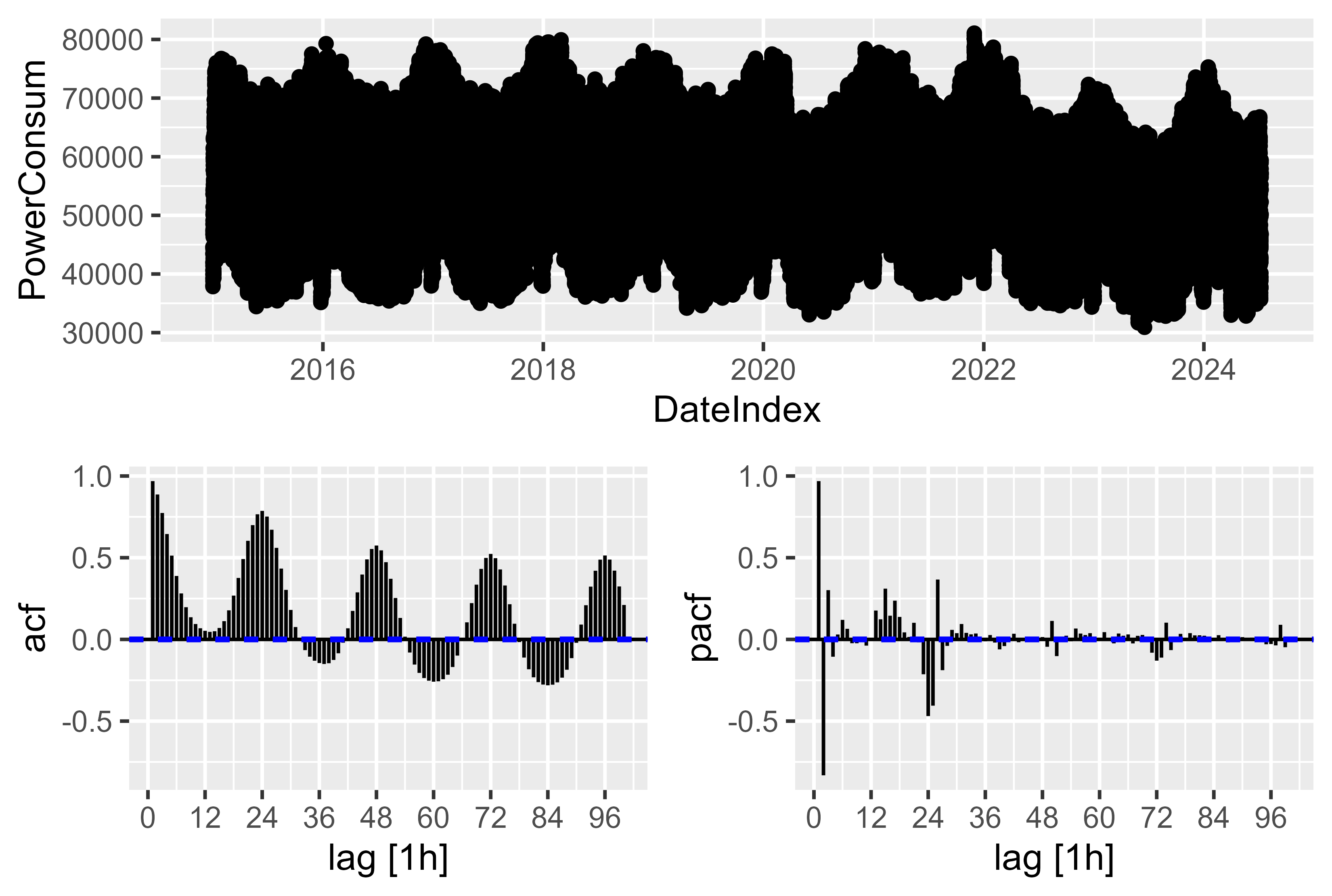 圖 12 功耗 - ACF PACF 原始功耗圖
這項工作中發現的最佳功能組合是:
為了比較模型,我們使用 MAE 和 MAPE 指標。 SMARD 是 SMARD 頁面上「Bundesnetzagentur」的模型。 Prophet模型也被嘗試過,表現不錯,但還不夠好。
SMARD 預測值的 MAPE 達到 3.6%。 <- 不在本研究中。
訓練資料:
迄今為止發現的最好的模型是 LHM + DHR(線性諧波模型 + 動態諧波回歸)
這個想法是將線性模型與 ARIMA 模型整合。因為 ARIMA 模型很難處理假期的虛擬變數。因此,集成模型發揮了作用。
 train_power_consum <- cleaned_power_consum |>
    filter(year(DateIndex) > 2020 & (year(DateIndex) < 2024))

generate_models(model_name = "model/mean_naive_drift",
                train_power_consum = train_power_consum)

train_power_consum_v5 <- train_power_consum |>
  mutate(HolidaySmoothed = Holiday + sin(2 * pi * (as.numeric(Hour)+1) / 24))

holiday_effect_model <- lm(
  PowerConsum ~
    HolidaySmoothed,
  data = train_power_consum_v5
)

saveRDS(holiday_effect_model, file = "ensemble_model/version_5/holiday_effect_2021_2023.rds")

train_power_consum_v5$Residuals <- residuals(holiday_effect_model)

fit <- train_power_consum_v5 |>
  model(
    ARIMA = ARIMA(Residuals ~
                    PDQ(0,0,0)
                  + pdq(d=0)
                  + MeanLastWeek
                  + WorkDay
                  + EndOfTheYear # new
                  + FirstWeekOfTheYear # new
                  + MeanLastTwoDays
                  + MaxLastOneDay
                  + MinLastOneDay
                  + fourier(period = "day", K = 6)
                  + fourier(period = "week", K = 7)
                  + fourier(period = "year", K = 3)
    )
  )

saveRDS(fit, file = "ensemble_model/version_5/arima_2021_2023.rds")
我們可以直觀地看到效果以及模型的工作原理。圖 13 顯示了該模型背後的想法。首先,我們擬合 LHM 模型並計算殘差。透過殘差訓練 DHR 模型並對兩者求和。它有點像 LHM 上的鏡像,並將值推回頂部。
對於 LHM 模型,我們在這裡使用一種簡單的方法,即每 24 小時重複一次的正弦曲線,並在假期或工作日減少或增加。
透過預測新資料的 LHM,我們可以預測新資料的殘差。殘差 + LHM 將數值移回「正確」位置。
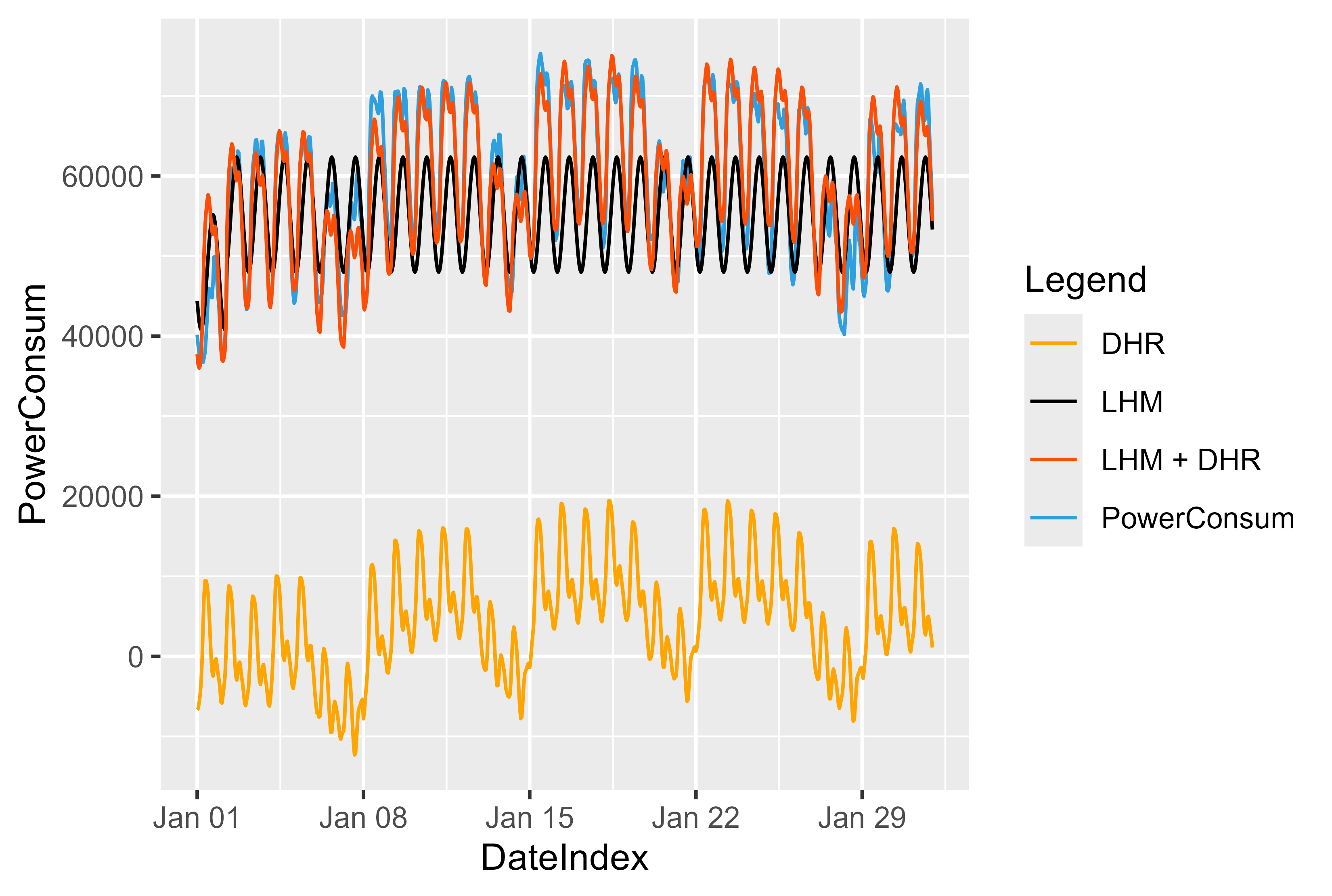 圖 13 LHM + DHR 模型表示
 ensembled_fc <- load_ensembled_models(
  days_to_forecast = 40,
  months_to_forecast = 6,
  year_to_forecast = 2024,
  starting_month = 1,
  real_data = cleaned_power_consum,
  smard_fc = cleaned_smard_pred,
  model_path = "ensemble_model"
)
all_forecasts_ensembled <- ensembled_fc$all_forecasts
raw_fc_ensembled <- ensembled_fc$raw_forecasts

fc <- load_all_model_results(
  days_to_forecast = 40,
  months_to_forecast = 6,
  year_to_forecast = 2024,
  starting_month = 1,
  smard_fc = cleaned_smard_pred,
  real_data = cleaned_power_consum
)

all_forecasts <- fc$combined_forecasts
raw_fc <- fc$raw_forecasts


metric_results <- calculate_metrics(fc_data = all_forecasts, fc_data_ensembled=all_forecasts_ensembled)

# Plot best Model for single Models
name_of_best_model_for_single_model <- plot_forecast(
  all_forecasts = all_forecasts,
  metric_results = metric_results,
  cleaned_power_consum = cleaned_power_consum,
  raw_fc = raw_fc,
  month_to_plot = 1,
  days_to_plot = 40
)

# Plot best Model for ensembled Models
name_of_best_model_ensembled <- plot_forecast_ensembled(
  all_forecasts = all_forecasts_ensembled,
  metric_results = metric_results,
  cleaned_power_consum = cleaned_power_consum,
  month_to_plot = 1,
  days_to_plot = 40
)

# Residuals Compared with SMARD
plot_compare_with_smard(
  all_forecasts = all_forecasts_ensembled,
  name_of_best_model = name_of_best_model_ensembled
  )


# LHM DHM representation
plot_representation_of_lhm_dhm_components(path_dhm = "ensemble_model/version_5/arima_2021_2023.rds",
                                          path_lhm = "ensemble_model/version_5/holiday_effect_2021_2023.rds",
                                          from_month = 1,
                                          to_month = 1,
                                          raw_fc_ensembled = raw_fc_ensembled)
version_5(LHM + DHR 模型)的 MAPE 得分為 3.8%。
讓我們更深入地了解是否僅使用 ARIMA 模型 (arima_14)。圖 14 展示了該模型的結果。我們可以看到假日(橙色)、週末(紅色)和正常日期(藍色)。假期有顯著的異常值,儘管 ARIMA 模型有一個虛擬變量,但它無法正確捕捉假期。
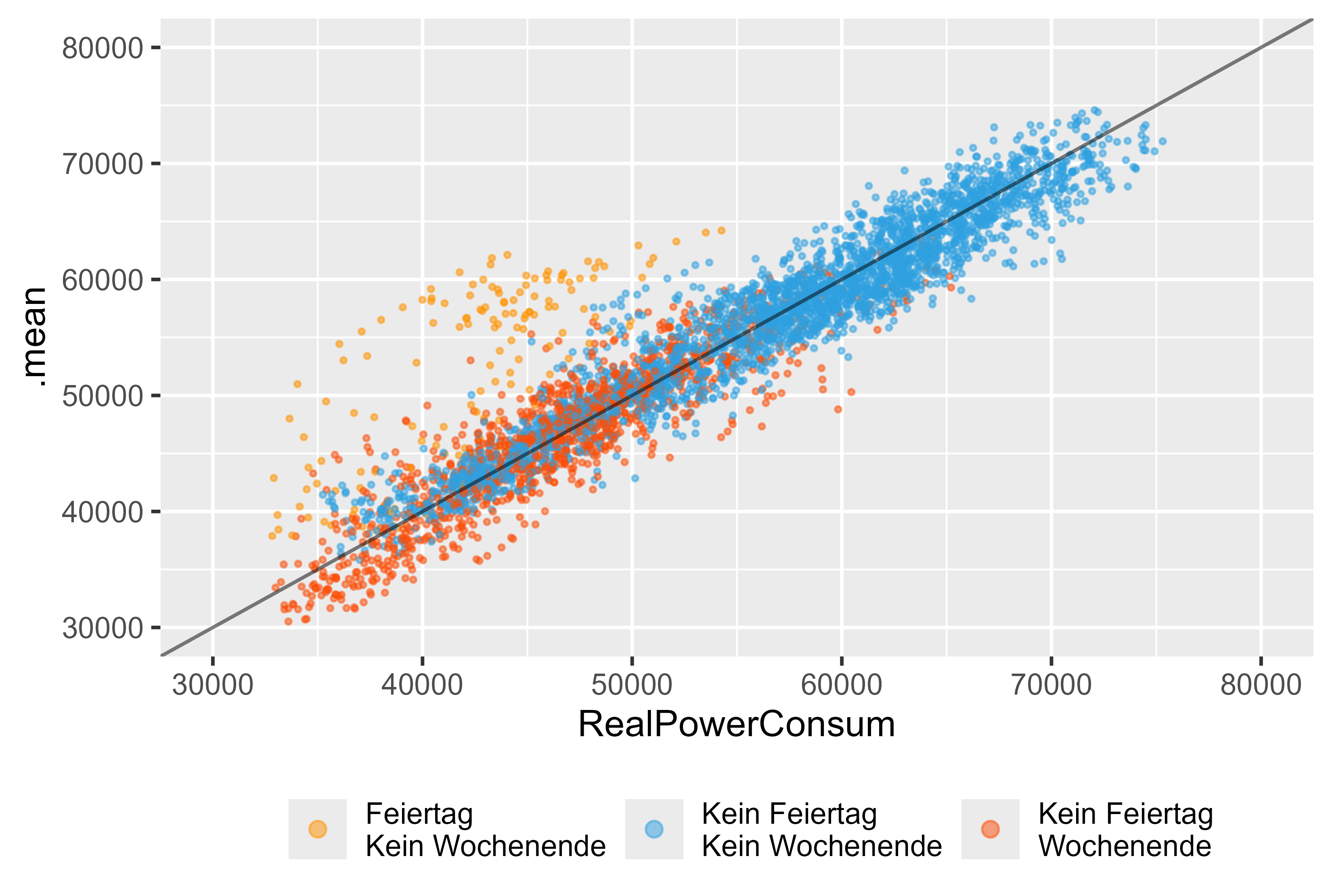 圖 14 預測與實際值 ARIMA(DHR、arima_14),作為單一模型
另一方面,LHM + DHR 模型在假期中表現更好。圖 15 代表了它。
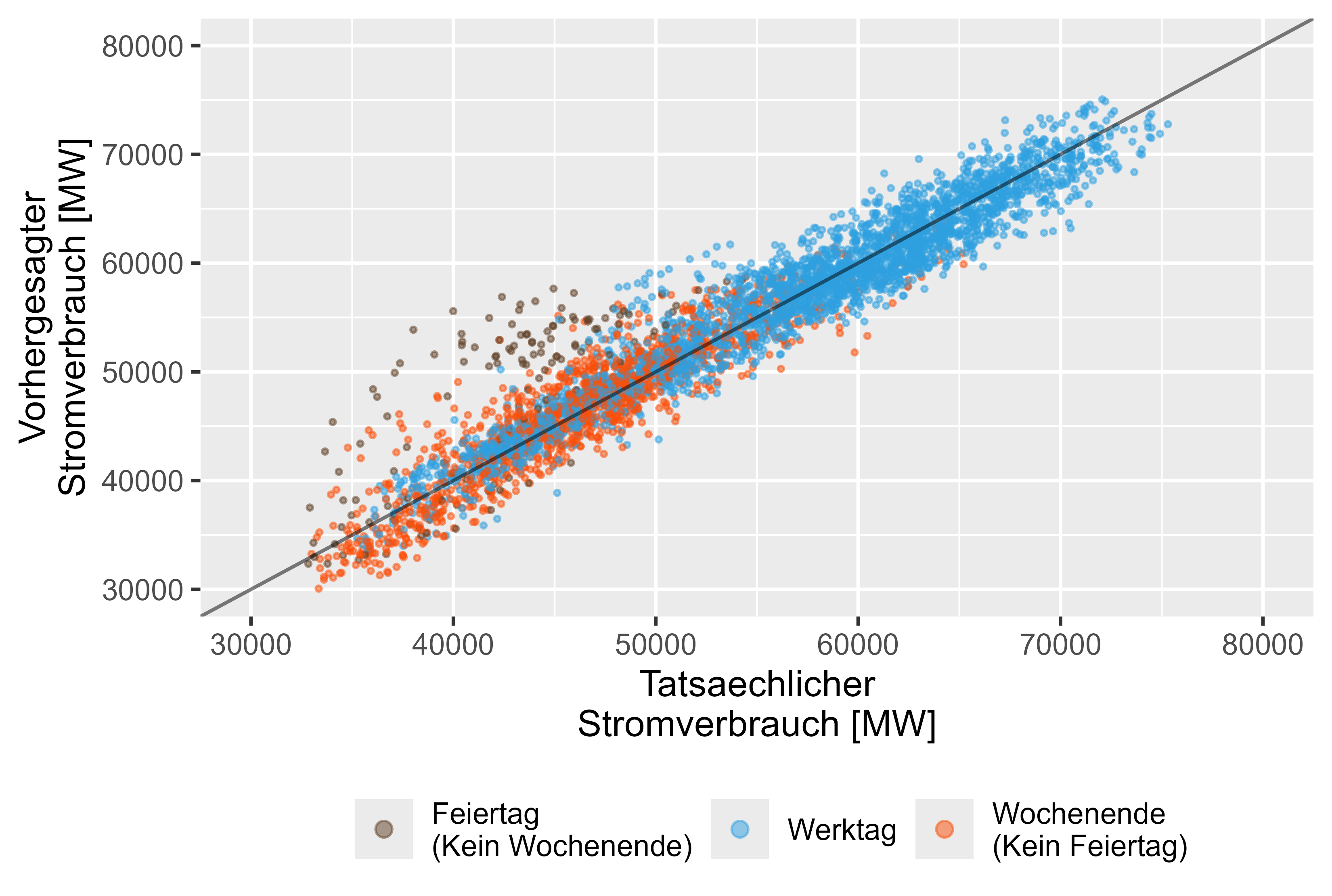 圖 15 預測與實際值 LHM + DHR,整合模型
圖 16 顯示了 2024 年 1 月的預測。
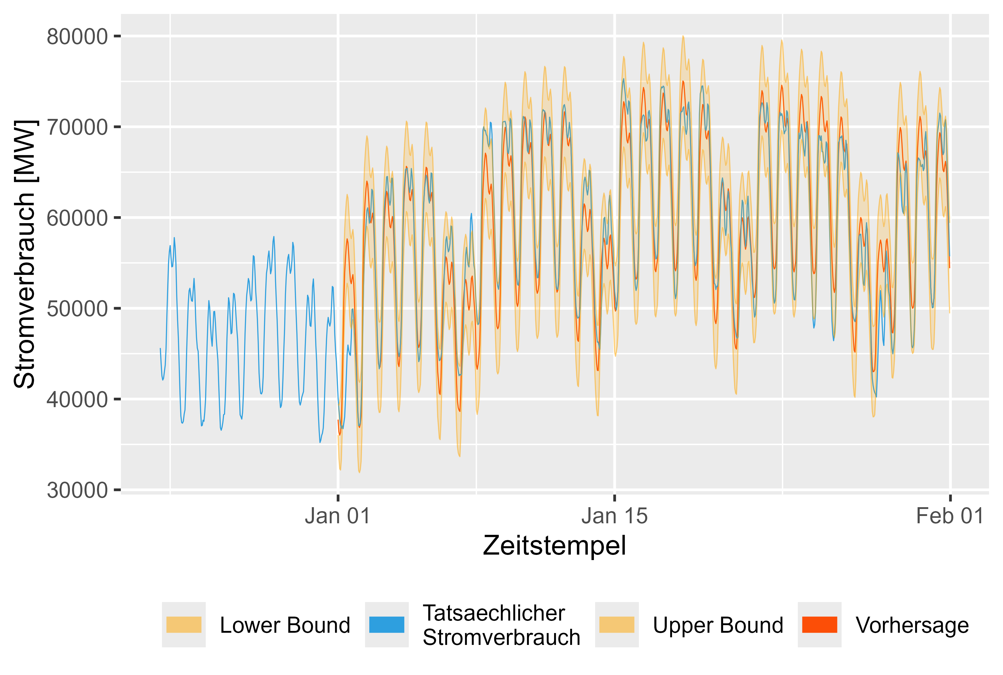 圖 16 2024 年 1 月預測值與實際值 LHM + DHR
此外,與 SMARD 模型相比,該模型的殘差看起來也不錯。很少有峰值,但可能很重要,並且可以透過建模更好地準備。但總體而言,這是一個堅實的結果。
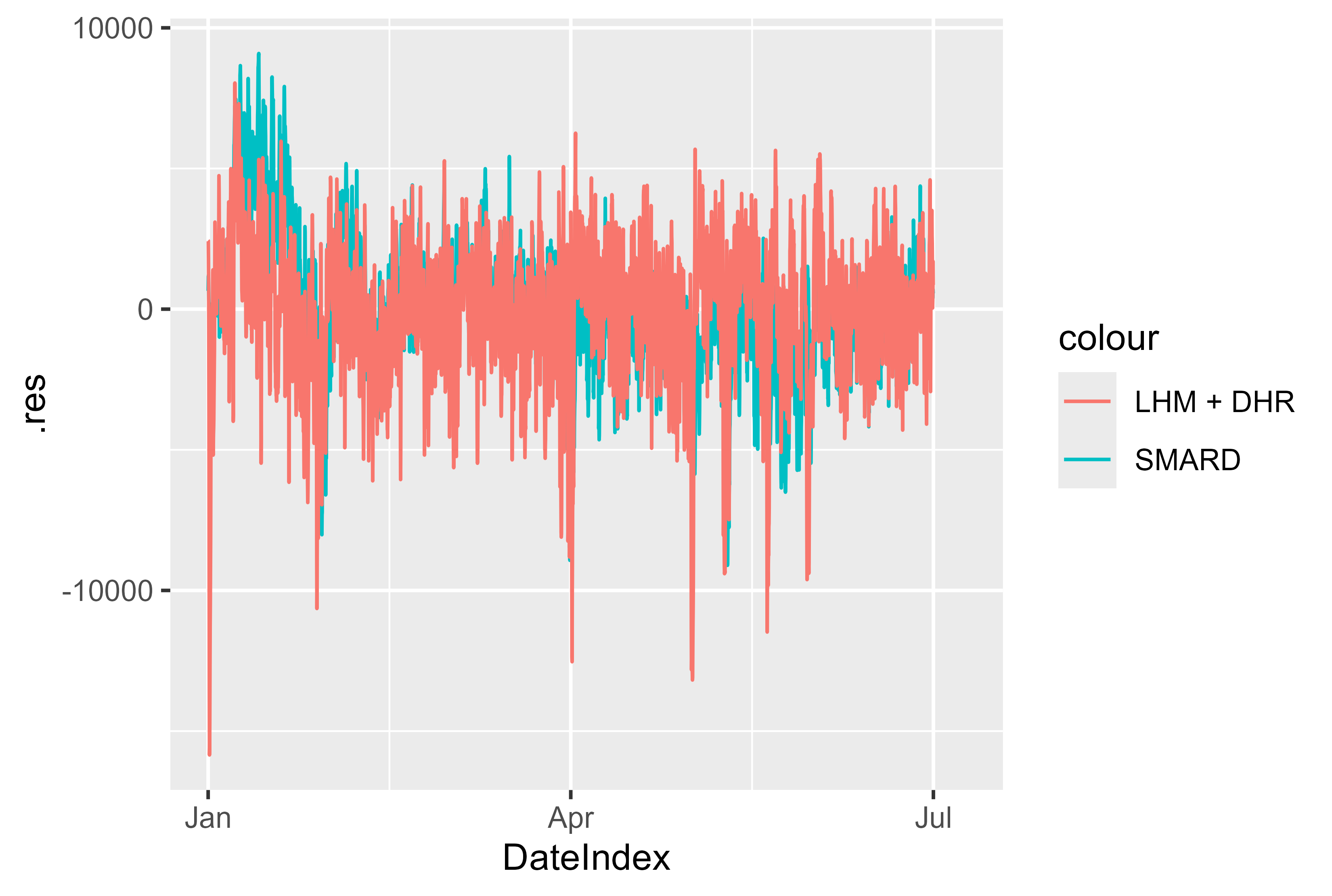 圖 17 2024 年 1 月 - 7 月的殘差 LHM + DHR
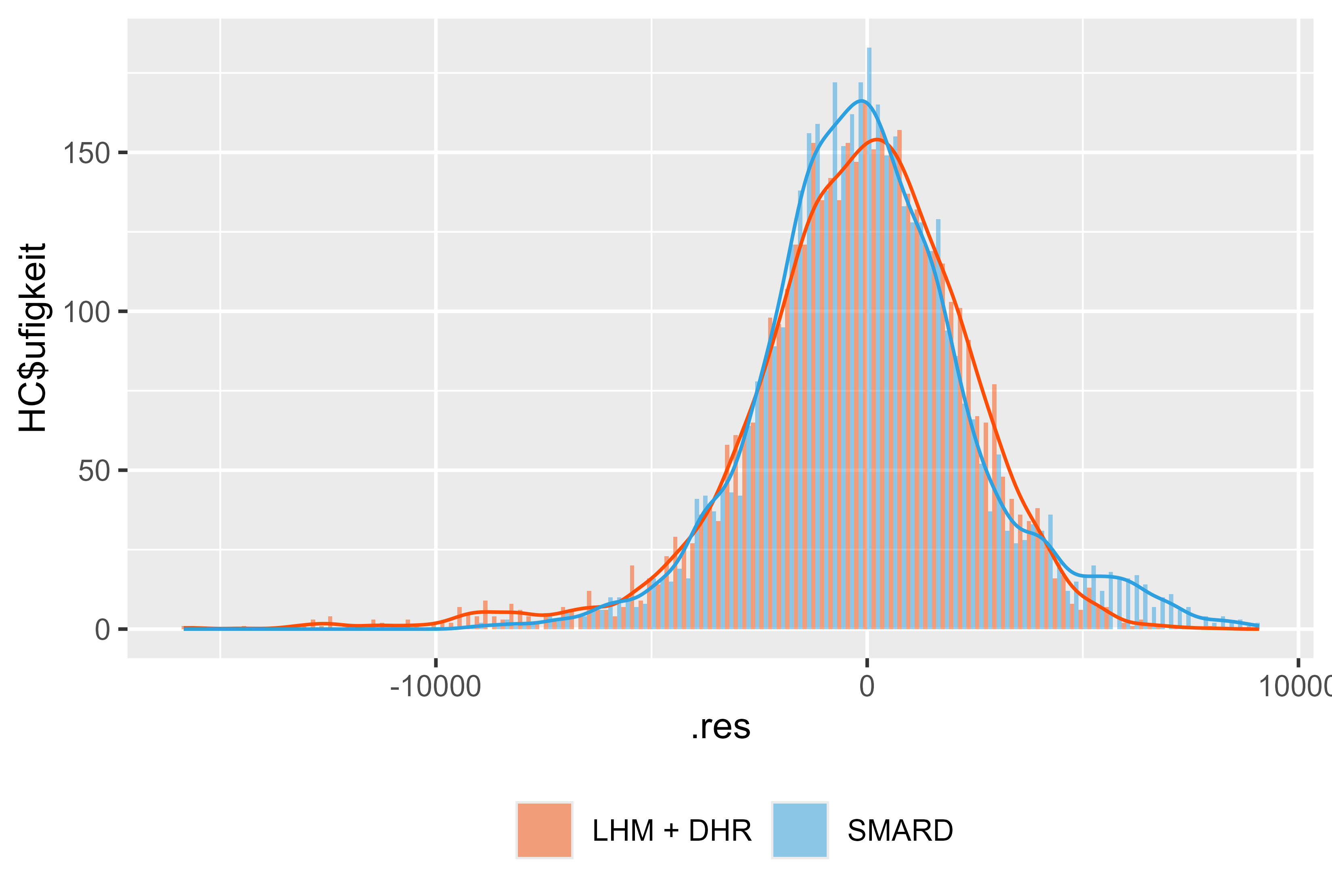 圖 18 2024 年 1 月 - 7 月的殘差 LHM + DHR
| 指數 | 型號名稱 | 均方根誤差 | MAPE | MAE | 合奏 |
|---|---|---|---|---|---|
| 2 | 真實觀察 | 0.000 | 0.000000 | 0.000 | 真的 |
| 3 | SMARD | 2480.693 | 3.602140 | 1869.466 | 錯誤的 |
| 4 | SMARD | 2480.693 | 3.602140 | 1869.466 | 真的 |
| 5 | 版本_5 | 2626.807 | 3.816012 | 1937.670 | 真的 |
| 6 | 版本_0 | 2613.258 | 3.846888 | 1946.314 | 真的 |
| 7 | 版本_7 | 2770.359 | 4.107272 | 2076.045 | 真的 |
| 8 | 版本_8 | 2775.441 | 4.146788 | 2091.153 | 真的 |
| 9 | 版本_9 | 2887.179 | 4.177841 | 2100.381 | 真的 |
| 10 | 版本_6 | 2906.242 | 4.216517 | 2142.092 | 真的 |
| 11 | arima_14_2021_2023.rds | 3208.735 | 4.389492 | 2207.395 | 錯誤的 |
| 12 | arima_18_2021_2023.rds | 3208.735 | 4.389492 | 2207.395 | 錯誤的 |
| 13 | 版本_4 | 2875.929 | 4.535388 | 2255.645 | 真的 |
| 14 | 版本_2 | 2905.990 | 4.580770 | 2279.624 | 真的 |
| 15 | arima_9_2021_2023.rds | 3267.160 | 4.611857 | 2302.918 | 錯誤的 |
| 16 | arima_2_2021_2023.rds | 3251.390 | 4.614028 | 2301.447 | 錯誤的 |
| 17 號 | arima_4_2021_2023.rds | 3251.390 | 4.614028 | 2301.447 | 錯誤的 |
| 18 | arima_5_2021_2023.rds | 3251.390 | 4.614028 | 2301.447 | 錯誤的 |
| 19 | arima_13_2021_2023.rds | 3283.745 | 4.619636 | 2307.415 | 錯誤的 |
| 20 | arima_10_2021_2023.rds | 3265.913 | 4.625508 | 2314.395 | 錯誤的 |
| 21 | arima_0_2021_2023.rds | 3269.009 | 4.645944 | 2317.138 | 錯誤的 |
| 22 | arima_17_2021_2023.rds | 3269.009 | 4.645944 | 2317.138 | 錯誤的 |
| 23 | arima_16_2021_2023.rds | 3298.902 | 4.673116 | 2334.857 | 錯誤的 |
| 24 | arima_1_2021_2023.rds | 3312.429 | 4.696342 | 2340.193 | 錯誤的 |
| 24 | Prophet_0_2021_2023.rds | 3044.849 | 4.711527 | 2435.572 | 錯誤的 |
| 25 | arima_8_2021_2023.rds | 3332.217 | 4.716612 | 2358.085 | 錯誤的 |
| 26 | arima_11_2021_2023.rds | 3358.020 | 4.758970 | 2388.791 | 錯誤的 |
| 27 | arima_12_2021_2023.rds | 3430.191 | 5.022772 | 2495.067 | 錯誤的 |
| 28 | arima_7_2021_2023.rds | 3475.671 | 5.049287 | 2510.903 | 錯誤的 |
| 29 | 版本_3 | 3546.729 | 5.064654 | 2570.530 | 真的 |
| 30 | arima_15_2021_2023.rds | 3734.584 | 5.165147 | 2606.661 | 錯誤的 |
| 31 | arima_6_2021_2023.rds | 3748.583 | 5.375326 | 2723.837 | 錯誤的 |
| 32 | 版本_1 | 4495.568 | 6.483477 | 3229.647 | 真的 |
| 33 | arima_3_2021_2023.rds | 4558.982 | 6.953247 | 3453.387 | 錯誤的 |
| 34 | tslm_0_2021_2023.rds | 6760.994 | 11.189119 | 5694.949 | 錯誤的 |
| 35 | mean_2021_2023.rds | 9489.303 | 16.406032 | 8101.476 | 錯誤的 |
| 36 | naive_2021_2023.rds | 14699.338 | 20.797370 | 12130.587 | 錯誤的 |
| 37 | drift_2021_2023.rds | 14763.692 | 20.917883 | 12200.002 | 錯誤的 |
筆記:
檢查 example/ensemble_model_2022_forecast 或 example/ensemble_model_2023_forecast
我們可以包括更多因素,例如: