Huawei UK University Challenge Competition 2021
1.0.0

團隊主持人: Kahraman Kostas
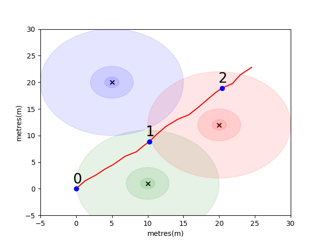
為了讓您開始,我們已經解決了一個簡單的問題,以引入一些關鍵的室內定位概念。考慮以下環境:在有3個WiFi發射器的情況下,用戶正在開放空間中行駛(我們將本用戶創建的數據稱為軌跡)。每個發射器都有一個唯一的MAC地址。用戶配備了一款智能手機,該智能手機將定期掃描WiFi環境並記錄每個檢測到的Mac(以DB)的RSSI。
對於此模型,我們為每個發射器使用了標準的日誌自由空間傳播模型。這是一個簡單的模型,可在自由空間中效果很好,但是在帶有牆壁和其他障礙物的實際室內環境中分解,可以以更複雜的方式反彈信號。通常,隨著發射天線的固定能量分佈在增加的區域,隨著波浪的傳播,我們確實希望RSSI在距離上急劇下降。在下面的圖中,每個圓表示下降的10dB。
用戶從點(0,0)上向東北行走,那裡的電話進行了三個環境掃描。每次掃描記錄的數據如下所示。
 scan 0 -> {'green': -60, 'blue': -66, 'red': -67}
scan 1 -> {'green': -58, 'blue': -61, 'red': -60}
scan 2 -> {'green': -66, 'blue': -62, 'red': -59}
WiFi環境的複雜且本地獨特的特性使其對於室內定位系統非常有用。例如,在下圖中,圖像scan 1在三個發射器的質心上測量數據,並且在這種環境中沒有其他位置可以進行讀取相似的RSSI值。考慮到來自獨立軌蹟的一組掃描或“指紋”,我們有興趣計算它們在WiFi空間中的相似程度,因為這表明它們在真實空間中的距離有多近。
您的第一個挑戰是編寫一個函數,以計算我們上面引入的樣品軌跡中的每個掃描之間的歐幾里得距離和曼哈頓距離指標。使用來自單個軌蹟的數據是測試相似性度量質量的好方法,因為我們可以使用手機的互助測量單元(IMU)獲得相當準確的真實距離估算,該數據由行人死亡估算使用,該單元使用該數據( PDR)模塊。
 def euclidean ( fp1 , fp2 ):
    raise NotImplementedError

def manhattan ( fp1 , fp2 ):
    raise NotImplementedError
# solution of the above functions
from scipy . spatial import distance
def euclidean ( fp1 , fp2 ):
fp1 = list ( fp1 . values ())
fp2 = list ( fp2 . values ())
return distance . euclidean ( fp1 , fp2 )
def manhattan ( fp1 , fp2 ):
fp1 = list ( fp1 . values ())
fp2 = list ( fp2 . values ())
return distance . cityblock ( fp1 , fp2 ) import json
import numpy as np
import matplotlib . pyplot as plt
from metrics import eval_dist_metric
with open ( "intro_trajectory_1.json" ) as f :
traj = json . load ( f )
## Pre-calculate the pair indexes we are interested in
keys = []
for fp1 in traj [ 'fps' ]:
for fp2 in traj [ 'fps' ]:
# only calculate the upper triangle
if fp1 [ 'step_index' ] > fp2 [ 'step_index' ]:
keys . append (( fp1 [ 'step_index' ], fp2 [ 'step_index' ]))
## Get the distances from PDR
true_d = {}
for step1 in traj [ 'steps' ]:
for step2 in traj [ 'steps' ]:
key = ( step1 [ 'step_index' ], step2 [ 'step_index' ])
if key in keys :
true_d [ key ] = abs ( step1 [ 'di' ] - step2 [ 'di' ])
euc_d = {}
man_d = {}
for fp1 in traj [ 'fps' ]:
for fp2 in traj [ 'fps' ]:
key = ( fp1 [ 'step_index' ], fp2 [ 'step_index' ])
if key in keys :
euc_d [ key ] = euclidean ( fp1 [ 'profile' ], fp2 [ 'profile' ])
man_d [ key ] = manhattan ( fp1 [ 'profile' ], fp2 [ 'profile' ])
print ( "Euclidean Average Error" )
print ( f' { eval_dist_metric ( euc_d , true_d ):.2f } ' )
print ( "Manhattan Average Error" )
print ( f' { eval_dist_metric ( man_d , true_d ):.2f } ' ) Euclidean Average Error
9.29
Manhattan Average Error
4.90
如果您正確地實施了功能,則應該看到歐幾里得公制的平均誤差為9.29 ,而曼哈頓僅為4.90 。因此,對於此數據,曼哈頓距離是對真實距離的更好估計。
當然,這是一個非常簡單的模型。確實,以這種方式,RSSI值與自由空間距離之間沒有直接的關係。通常,當我們創建自己的距離估計值時,我們將使用軌跡內的已知PDR距離將數字得分擬合到物理距離估計值。
對於您的主要挑戰,我們希望您開發自己的指標,以估算兩次掃描之間的現實世界距離,僅基於其WiFi指紋。我們將為您提供2021年初從一個購物中心收集的真正眾包數據。數據將包含114661指紋掃描和掃描之間的879824距離。距離將是我們將考慮的其他信息的最佳估計。
我們將提供一組指紋對的測試集,您需要編寫一個函數,告訴我們它們的相距多遠。
該功能可能就像我們上面介紹的一個指標之一一樣簡單,也可以像完整的機器學習解決方案一樣複雜,該解決方案在不同情況下學會了對不同的MAC地址(或MAC地址組合)的加權不同。
要考慮的一些最後點:
數據將作為您的三個文件組裝。
task1_fingerprints.json包含問題的所有指紋信息。那就是每個條目代表購物中心區域中WiFi發射器的真實掃描。您會發現許多指紋中都會存在相同的MAC地址。
task1_train.csv包含有效的培訓對,以幫助您設計/訓練算法。每個id1-id2對具有一個標記的地面真相距離(以米為單位),每個ID對應於task1_fingerprints.json的指紋。
task1_test.csv格式與task1_train.csv格式相同,但沒有包含的位移。這些是我們希望您使用原始指紋信息預測的內容。
 import csv
import json
import os
from tqdm import tqdm

path_to_data = "for_contestants"

with open ( os . path . join ( path_to_data , "task1_fingerprints.json" )) as f :
    fps = json . load ( f )

with open ( os . path . join ( path_to_data , "task1_train.csv" )) as f :
    train_data = []
    train_h = csv . DictReader ( f )
    for pair in tqdm ( train_h ):
        train_data . append ([ pair [ 'id1' ], pair [ 'id2' ], float ( pair [ 'displacement' ])])

with open ( os . path . join ( path_to_data , "task1_test.csv" )) as f :
    test_h = csv . DictReader ( f )
    test_ids = []
    for pair in tqdm ( test_h ):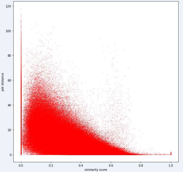
test_ids . append ([ pair [ 'id1' ], pair [ 'id2' ]])最終,理想的模型應該能夠在高度尺寸的指紋空間(1指紋可以包含許多測量值)和1維距離空間之間找到精確的映射。將PDR距離(與培訓數據)繪製在某些計算的相似性度量上,以查看該度量是否揭示出明顯的趨勢可能是有用的。高相似性應與低距離相關。
以下是我們內部用於此任務的一個距離指標。您可以看到,即使對於這個指標,我們也有大量的噪音。
由於這種噪音水平,我們的任務1的評分指標將偏向於精確度而不是召回
您的提交應使用test1_test.csv文件中的確切ID,並應使用該指紋對的估計距離(以米為單位)填充第三個(當前空)位移列。
 def my_distance_function ( fp1 , fp2 ):
    raise NotImplementedError
output_data = [[ "id1" , "id2" , "displacement" ]]
for id1 , id2 in tqdm ( test_ids ):
fp1 = fps [ id1 ]
fp2 = fps [ id2 ]
distance_estimate = my_distance_function ( fp1 , fp2 )
output_data . append ([ id1 , id2 , distance_estimate ])
with open ( "MySubmission.csv" , "w" , newline = '' ) as f :
writer = csv . writer ( f )
writer . writerows ( output_data )第一個任務中的步驟可以匯總如下。
這些步驟在下圖中說明。
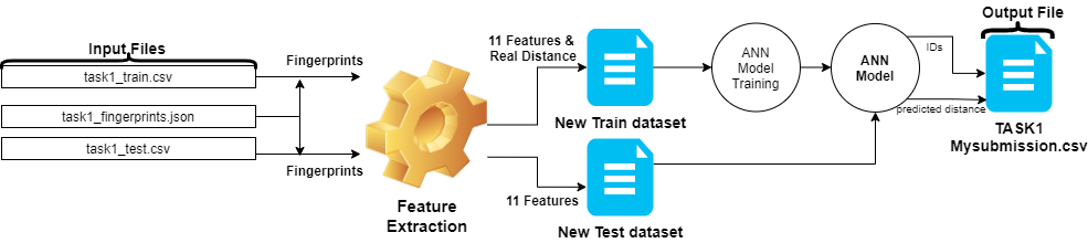
我們使用Python 3.6.5創建應用程序文件。我們包括了一些其他模塊,這些模塊未包含在比賽開始時給出的示例文件中。這些模塊可以列為:
| molules | 任務 |
|---|---|
| 張量 | 深度學習 |
| 貓熊 | 數據分析 |
| Scipy | 距離計算 |
我們從安裝這些模塊作為第一步。
 ## 1.1 Installing modules
!p ip install tensorflow == 2.6 . 2
!p ip install scipy
!p ip install pandas 在此步驟中,我們修復了相關的隨機種子以獲得可重複的結果。這樣,我們提供了一個確定性的路徑,在每次運行中都會獲得相同的結果。但是,根據我們的觀察,用不同計算機獲得的結果可能略有不同(±1%)
 ## 1.2  Setting Random Seeds
seed_value = 0

import os
os . environ [ 'PYTHONHASHSEED' ] = str ( seed_value )

import random
random . seed ( seed_value )

import numpy as np
np . random . seed ( seed_value )

import tensorflow as tf
tf . random . set_seed ( seed_value )

import tensorflow as tf

session_conf = tf . compat . v1 . ConfigProto ( intra_op_parallelism_threads = 1 , inter_op_parallelism_threads = 1 )
sess = tf . compat . v1 . Session ( graph = tf . compat . v1 . get_default_graph (), config = session_conf )在本節中,我們加載了將使用的數據。我們從給出的示例文件( Task1-IPS-Challenge-2021.ipynb )中獲取了代碼和說明。
task1_fingerprints.json包含問題的所有指紋信息。那就是每個條目代表購物中心區域中WiFi發射器的真實掃描。您會發現許多指紋中都會存在相同的MAC地址。
task1_train.csv包含有效的培訓對,以幫助您設計/訓練算法。每個id1-id2對具有一個標記的地面真相距離(以米為單位),每個ID對應於task1_fingerprints.json的指紋。
task1_test.csv格式與task1_train.csv格式相同,但沒有包含的位移。
 ## 1.3 Loading the data
import csv
import json
import os
from tqdm import tqdm

path_to_data = "for_contestants"

with open ( os . path . join ( path_to_data , "task1_fingerprints.json" )) as f :
    fps = json . load ( f )

with open ( os . path . join ( path_to_data , "task1_train.csv" )) as f :
    train_data = []
    train_h = csv . DictReader ( f )
    for pair in tqdm ( train_h ):
        train_data . append ([ pair [ 'id1' ], pair [ 'id2' ], float ( pair [ 'displacement' ])])

with open ( os . path . join ( path_to_data , "task1_test.csv" )) as f :
    test_h = csv . DictReader ( f )
    test_ids = []
    for pair in tqdm ( test_h ):
        test_ids . append ([ pair [ 'id1' ], pair [ 'id2' ]])
879824it [05:16, 2778.31it/s]
5160445it [01:00, 85269.27it/s]
在此步驟中,我們使用兩個功能執行特徵提取。 feature_extraction_file函數只需從JSON文件中拉出指紋的相關值(成對),然後將它們發送到feature_extraction函數以進行計算。
在feature_extraction函數中,如果這兩個指紋在尺寸和所包含的設備方面相互不同,則將兩個指紋中包含的所有設備匯集在一起以形成一個常見的序列而無需重複。在每個數組中,我們通過將值0分配給非相應的設備來使這兩個數組(以它們包含的設備為方面)相同。以下圖像中的一個示例對此過程進行了解釋。
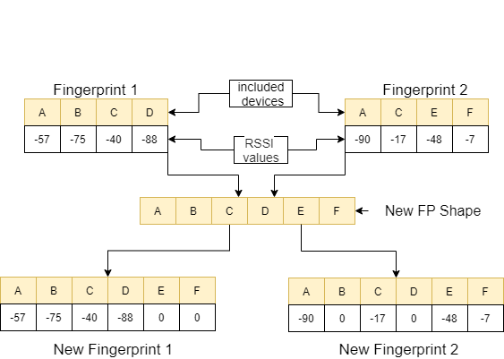
這兩個指紋之間的距離使用11種不同的方法進行了計算[1]。這些方法是:
然後,將這些值定向到feature_extraction_file函數,並在此函數中保存為CSV文件。換句話說,由於此過程,各種尺寸的指紋變成了11-曲的CSV文件。使用這些新創建的功能對要使用的模型進行了訓練和測試。
 ## 1.4 Feature Extraction

def feature_extraction_file ( data , name , flag ):
    features = [[ "braycurtis" ,
    "canberra" ,
    "chebyshev" ,
    "cityblock" ,
    "correlation" ,
    "cosine" ,
    "euclidean" ,
    "jensenshannon" ,
    "minkowski" ,
    "sqeuclidean" ,
    "wminkowski" , "real" ]]
    for i in tqdm (( data ), position = 0 , leave = True ):
        fp1 = fps [ i [ 0 ]]
        fp2 = fps [ i [ 1 ]]
        feature = feature_extraction ( fp1 , fp2 )
        if flag :
            feature . append ( i [ 2 ])
        else : feature . append ( 0 )
        features . append ( feature )
    with open ( name , "w" , newline = '' ) as f :
        writer = csv . writer ( f )
        writer . writerows ( features )
    #print(features)
## 1.4 Feature Extraction
def feature_extraction ( fp1 , fp2 ):
mac = set ( list ( fp1 . keys ()) + list ( fp2 . keys ()))
mac = { i : 0 for i in mac }
f1 = mac . copy ()
f2 = mac . copy ()
for key in fp1 :
f1 [ key ] = fp1 [ key ]
for key in fp2 :
f2 [ key ] = fp2 [ key ]
f1 = list ( f1 . values ())
f2 = list ( f2 . values ())
braycurtis = scipy . spatial . distance . braycurtis ( f1 , f2 )
canberra = scipy . spatial . distance . canberra ( f1 , f2 )
chebyshev = scipy . spatial . distance . chebyshev ( f1 , f2 )
cityblock = scipy . spatial . distance . cityblock ( f1 , f2 )
correlation = scipy . spatial . distance . correlation ( f1 , f2 )
cosine = scipy . spatial . distance . cosine ( f1 , f2 )
euclidean = scipy . spatial . distance . euclidean ( f1 , f2 )
jensenshannon = scipy . spatial . distance . jensenshannon ( f1 , f2 )
minkowski = scipy . spatial . distance . minkowski ( f1 , f2 )
sqeuclidean = scipy . spatial . distance . sqeuclidean ( f1 , f2 )
wminkowski = scipy . spatial . distance . wminkowski ( f1 , f2 , 1 , np . ones ( len ( f1 )))
output_data = [ braycurtis ,
canberra ,
chebyshev ,
cityblock ,
correlation ,
cosine ,
euclidean ,
jensenshannon ,
minkowski ,
sqeuclidean ,
wminkowski ]
output_data = [ 0 if x != x else x for x in output_data ]
return output_data 在此任務中,有指紋掃描,這些掃描具有來自購物中心WiFi發射器周圍環境的RRSI信號。首先,挑戰希望我們估計兩種指紋掃描之間的距離,這是回歸任務。我們使用了受生物神經網絡啟發的ANN(人工神經網絡)。安由三層組成;輸入層,隱藏圖層(多個)和輸出層。 ANN從輸入層開始,其中包括訓練數據(帶有功能),將數據傳遞到第一個隱藏層,該隱藏層由第一個隱藏層的權重計算出數據。在隱藏的層中,重量的重量計算到輸入中,然後將它們應用於激活函數[2]。由於我們的問題是回歸,我們的最後一層是一個單個輸出神經元:其輸出是指紋掃描對之間的距離。我們的第一個隱藏層具有64個,第二層具有128個神經元。該模型的所有架構如下。 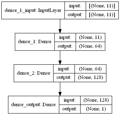
我們使用兩個功能進行深度學習。create_model create_model塑造了訓練數據以訓練模型並確定模型的結構。 model_features函數可產生具有指定結構的模型。通過create_model函數訓練後,可以保存創建的模型。
## 1.5 Model
import scipy . spatial
import pandas as pd
import numpy as np
import matplotlib . pyplot as plt
from tensorflow import keras
from tensorflow . keras . models import Sequential
from tensorflow . keras . layers import Dense
#from keras.utils.vis_utils import plot_model
% matplotlib inline
def model_features ( i , ii ):
model = Sequential ()
model . add ( Dense ( i , input_shape = ( 11 , ), activation = 'relu' , name = 'dense_1' ))
model . add ( Dense ( ii , activation = 'relu' , name = 'dense_2' ))
model . add ( Dense ( 1 , activation = 'linear' , name = 'dense_output' ))
model . compile ( optimizer = 'adam' , loss = 'mse' , metrics = [ 'mae' ])
model . summary ()
#plot_model(model, to_file='model_plot.png', show_shapes=True, show_layer_names=True)
#print(model.get_config())
return model
def create_model ( name ):
df = pd . read_csv ( name )
df . replace ([ np . inf , - np . inf ], np . nan , inplace = True )
df = df . fillna ( 0 )
X = df [ df . columns [ 0 : - 1 ]]
X_train = np . array ( X )
y_train = np . array ( df [ df . columns [ - 1 ]])
model = model_features ( 64 , 128 )
history = model . fit ( X_train , y_train , epochs = 19 , validation_split = 0.5 ) #,batch_size=1)
loss = history . history [ 'loss' ]
val_loss = history . history [ 'val_loss' ]
my_xticks = list ( range ( len ( loss )))
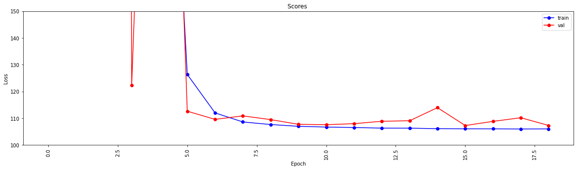
plt . figure ( figsize = ( 20 , 5 ))
plt . plot ( my_xticks , loss , linestyle = '-' , marker = 'o' , color = 'b' , label = "train" )
plt . plot ( my_xticks , val_loss , linestyle = '-' , marker = 'o' , color = 'r' , label = "val" )
plt . title ( "Scores " )
plt . legend ( numpoints = 1 )
plt . ylabel ( "Loss" )
plt . xlabel ( "Epoch" )
plt . xticks ( rotation = 90 )
plt . ylim ([ 100 , 150 ])
plt . show ()
madelname = "./THEMODEL"
model . save ( madelname )
print ( "Model Created!" )
此功能檢查訓練和測試數據是否通過功能提取。如果沒有,它可以通過調用相應的功能來創建這些文件和模型。處理模型和所有特徵提取後,它將測試數據格式化以產生最終結果。
 ## 1.6 Checking the inputs
from numpy import inf
from numpy import nan

def create_new_files ( train , test ):
    model_path = "./THEMODEL/"
    my_train_file = 'new_train_features.csv'
    my_test_file = 'new_test_features.csv'


    if os . path . isfile ( my_train_file ) :
        pass
    else :

        print ( "Please wait! Training data feature extraction is in progress... n it will take about 10 minutes" )
        feature_extraction_file ( train , my_train_file , 1 )
        print ( "TThe training feature extraction completed!!!" )


    if os . path . isfile ( my_test_file ) :
        pass
    else :

        print ( "Please wait! Testing data feature extraction is in progress... n it will take about 100-120 minutes" )
        feature_extraction_file ( test , my_test_file , 0 )
        print ( "The testing feature extraction completed!!!" )


    if  os . path . isdir ( model_path ):
        pass
    else :

        print ( "Please wait! Creating the deep learning model... n it will take about 10 minutes" )
        create_model ( my_train_file )
        print ( "The model file created!!! n n n " )

    model = keras . models . load_model ( model_path )
    df = pd . read_csv ( my_test_file )
    df . replace ([ np . inf , - np . inf ], np . nan , inplace = True )
    df = df . fillna ( 0 )
    X_train = df [ df . columns [ 0 : - 1 ]]
    X_train = np . array ( X_train )
    y_train = np . array ( df [ df . columns [ - 1 ]])
    predicted = model . predict ( X_train )
    print ( "Please wait! Creating resuşts... " )

return predicted 此步驟觸發器具有提取和模型創建過程,並允許所有過程開始。因此,使用test1_test.csv文件中的ID填充該指紋對的第三個(位移)列,並將此文件保存在目錄中,並使用名稱TASK1-MySubmission.csv 。
 ## 1.7 Submission
distance_estimate = create_new_files ( train_data , test_ids )
count = 0

output_data = [[ "id1" , "id2" , "displacement" ]]
for id1 , id2 in tqdm ( test_ids ):
    output_data . append ([ id1 , id2 , distance_estimate [ count ][ 0 ]])
    count += 1
print ( "Process finished. Preparing result file ..." )
with open ( "TASK1-MySubmission.csv" , "w" , newline = '' ) as f :
    writer = csv . writer ( f )
    writer . writerows ( output_data )
print ( "The results are ready. n See MySubmission.csv" )
Please wait! Creating the deep learning model...
it will take about 10 minutes
Model: "sequential_3"
_________________________________________________________________
Layer (type) Output Shape Param #
=================================================================
dense_1 (Dense) (None, 64) 768
_________________________________________________________________
dense_2 (Dense) (None, 128) 8320
_________________________________________________________________
dense_output (Dense) (None, 1) 129
=================================================================
Total params: 9,217
Trainable params: 9,217
Non-trainable params: 0
_________________________________________________________________
Epoch 1/19
13748/13748 [==============================] - 30s 2ms/step - loss: 2007233.6250 - mae: 161.3013 - val_loss: 218.8822 - val_mae: 11.5630
Epoch 2/19
13748/13748 [==============================] - 27s 2ms/step - loss: 24832.6309 - mae: 53.9385 - val_loss: 123437.0859 - val_mae: 307.2885
Epoch 3/19
13748/13748 [==============================] - 26s 2ms/step - loss: 4028.0859 - mae: 29.9960 - val_loss: 3329.2024 - val_mae: 49.9126
Epoch 4/19
13748/13748 [==============================] - 27s 2ms/step - loss: 904.7919 - mae: 17.6284 - val_loss: 122.3358 - val_mae: 6.8169
Epoch 5/19
13748/13748 [==============================] - 25s 2ms/step - loss: 315.7050 - mae: 11.9098 - val_loss: 404.0973 - val_mae: 15.2033
Epoch 6/19
13748/13748 [==============================] - 26s 2ms/step - loss: 126.3843 - mae: 7.8173 - val_loss: 112.6499 - val_mae: 7.6804
Epoch 7/19
13748/13748 [==============================] - 27s 2ms/step - loss: 112.0149 - mae: 7.4220 - val_loss: 109.5987 - val_mae: 7.1964
Epoch 8/19
13748/13748 [==============================] - 26s 2ms/step - loss: 108.6342 - mae: 7.3271 - val_loss: 110.9016 - val_mae: 7.6862
Epoch 9/19
13748/13748 [==============================] - 26s 2ms/step - loss: 107.6721 - mae: 7.2827 - val_loss: 109.5083 - val_mae: 7.5235
Epoch 10/19
13748/13748 [==============================] - 27s 2ms/step - loss: 107.0110 - mae: 7.2290 - val_loss: 107.7498 - val_mae: 7.1105
Epoch 11/19
13748/13748 [==============================] - 29s 2ms/step - loss: 106.7296 - mae: 7.2158 - val_loss: 107.6115 - val_mae: 7.1178
Epoch 12/19
13748/13748 [==============================] - 26s 2ms/step - loss: 106.5561 - mae: 7.2039 - val_loss: 107.9937 - val_mae: 6.9932
Epoch 13/19
13748/13748 [==============================] - 26s 2ms/step - loss: 106.3344 - mae: 7.1905 - val_loss: 108.8941 - val_mae: 7.4530
Epoch 14/19
13748/13748 [==============================] - 27s 2ms/step - loss: 106.3188 - mae: 7.1927 - val_loss: 109.0832 - val_mae: 7.5309
Epoch 15/19
13748/13748 [==============================] - 27s 2ms/step - loss: 106.1150 - mae: 7.1829 - val_loss: 113.9741 - val_mae: 7.9496
Epoch 16/19
13748/13748 [==============================] - 26s 2ms/step - loss: 106.0676 - mae: 7.1788 - val_loss: 107.2984 - val_mae: 7.2192
Epoch 17/19
13748/13748 [==============================] - 27s 2ms/step - loss: 106.0614 - mae: 7.1733 - val_loss: 108.8553 - val_mae: 7.4640
Epoch 18/19
13748/13748 [==============================] - 28s 2ms/step - loss: 106.0113 - mae: 7.1790 - val_loss: 110.2068 - val_mae: 7.6562
Epoch 19/19
13748/13748 [==============================] - 27s 2ms/step - loss: 106.0519 - mae: 7.1791 - val_loss: 107.3276 - val_mae: 7.0981
 INFO:tensorflow:Assets written to: ./THEMODELassets
Model Created!
The model file created!!!


Please wait! Creating resuşts...


100%|████████████████████████████████████████████████████████████████████| 5160445/5160445 [00:08<00:00, 610910.29it/s]


Process finished. Preparing result file ...
The results are ready.
 See MySubmission.csv
鑑於我們現在有一個用於評估WiFi距離的度量,但我們強烈建議一種圖形聚類方法。
將數據中的每個WiFi指紋視為圖中的節點,並且我們可以通過評估任何兩個指紋的相似性來與圖中的其他指紋形成邊緣。我們可以為指紋之間具有很高相似性的邊緣分配高的重量,而在不相似的邊緣之間具有很高的相似性和低重量(或沒有邊緣)。從理論上講,一個完全準確的相似性度量標準將在地板上微不足道地分開,因為我們可以排除大於4米(大約是建築物1層的高度)的所有邊緣。實際上,我們很可能會在樓層之間做出虛假的邊緣,我們需要以某種方式打破這些邊緣。
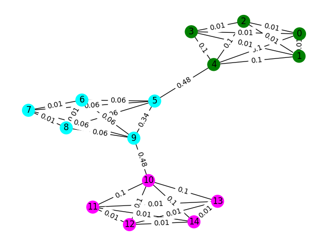
讓我們從一個簡單的示例開始。考慮下面的圖表,其中節點顏色顯示指紋的真實地板分類,邊緣反映出我們認為這些節點存在於同一地板上。在此練習中,我們已經預先標記了每個邊緣的“中間分數”,該度量可以計算出圖形中任何兩個節點之間的最短路徑來計算該邊緣的次數。通常,這將揭示表明高連通性的邊緣,並且可能是去除的候選者。
在此示例中,使用邊緣之間的分數來檢測圖形通信。返回一個列表,其中每個子列表包含社區的節點ID。請注意,這僅僅是為了幫助您理解問題,並且不計算實際解決方案。
 def detect_communities ( Graph ):
    ## This function should return a list of lists containing
    ## the node ids of the communities that you have detected.

    eb_score = nx . edge_betweenness_centrality ( G )

    raise NotImplementedError
import networkx as nx
from metrics import check_result
G = nx . read_adjlist ( "graph.adjlist" )
communities = detect_communities ( G )
if check_result ( communities ):
print ( "Correct!" )
else :
print ( "Try again" )此問題的樣本訓練數據是一組106981指紋( task2_train_fingerprints.json ),它們之間的一些邊緣。我們提供了指示三種不同邊緣類型的文件,所有這些都應以不同的方式處理。
task2_train_steps.csv指示在軌跡內連接後續步驟的邊緣。這些邊緣應高度信任,因為它們表明從同一樓層記錄了兩個指紋。
task2_train_elevations.csv表示步驟的相反。這些高程表明指紋幾乎肯定來自不同的地板。因此,如果指紋可以推斷
task2_train_estimated_wifi_distances.csv是我們使用自己的距離度量計算的預計距離。該指標是不完美的,因此我們知道許多這些邊緣將是不正確的(即它們將將兩層連接在一起)。我們建議您最初使用此文件中的邊緣來構建您的初始圖併計算一些解決方案。但是,如果您在Task1上獲得很高的分數,則可以考慮計算自己的WiFi距離以構建圖形。
您的圖形可以是兩個細節級別之一,即軌跡級別或指紋級別,您可以選擇要使用的表示形式,但最終我們想知道軌跡簇。軌跡水平將使每個節點作為軌跡,並且如果其軌跡中的指紋具有較高的相似性,則會發生節點之間的邊緣。指紋水平將每個指紋作為節點。您可以使用task2_train_lookup.json查找指紋的軌跡ID,以在表示之間轉換。
為了幫助您調試和訓練解決方案,我們為task2_train_GT.json中的某些軌跡提供了基礎真相。在此文件中,鍵是軌跡ID(與task2_train_lookup.json中的軌跡ID相同),並且值是建築物的真實地板ID。
測試集與訓練集完全相同的格式(對於單獨的建築物,我們不會使它變得容易;),但我們還沒有包括等效的地面真相文件。這將被禁止以允許我們為您的解決方案評分。
要考慮的要點
在本節中,我們將提供一些示例代碼來打開文件並構建兩種類型的圖形。
 import os
import json
import csv
import networkx as nx
from tqdm import tqdm

path_to_data = "task2_for_participants/train"

with open ( os . path . join ( path_to_data , "task2_train_estimated_wifi_distances.csv" )) as f :
    wifi = []
    reader = csv . DictReader ( f )
    for line in tqdm ( reader ):
        wifi . append ([ line [ 'id1' ], line [ 'id2' ], float ( line [ 'estimated_distance' ])])

with open ( os . path . join ( path_to_data , "task2_train_elevations.csv" )) as f :
    elevs = []
    reader = csv . DictReader ( f )
    for line in tqdm ( reader ):
        elevs . append ([ line [ 'id1' ], line [ 'id2' ]])

with open ( os . path . join ( path_to_data , "task2_train_steps.csv" )) as f :
    steps = []
    reader = csv . DictReader ( f )
    for line in tqdm ( reader ):
        steps . append ([ line [ 'id1' ], line [ 'id2' ], float ( line [ 'displacement' ])])

fp_lookup_path = os . path . join ( path_to_data , "task2_train_lookup.json" )
gt_path = os . path . join ( path_to_data , "task2_train_GT.json" )

with open ( fp_lookup_path ) as f :
    fp_lookup = json . load ( f )

with open ( gt_path ) as f :
    gt = json . load ( f )
這是構造指紋級圖的一種方法,其中圖中的每個節點都是指紋。我們添加了與WiFi和PDR邊緣的估計/真實距離相對應的邊緣權重。我們還添加了高程邊緣以表明這種關係。您可能需要明確強制執行開發解決方案時這些邊緣(或軌蹟之間的任何有效高程邊緣)。
 G = nx . Graph ()

for id1 , id2 , dist in tqdm ( steps ):
    G . add_edge ( id1 , id2 , ty = "s" , weight = dist )

for id1 , id2 , dist in tqdm ( wifi ):
    G . add_edge ( id1 , id2 , ty = "w" , weight = dist )

for id1 , id2 in tqdm ( elevs ):
G . add_edge ( id1 , id2 , ty = "e" )軌跡圖可以說不是您需要考慮的一種方法來表示軌蹟之間許多WiFi連接的方法。在下面的示例圖中,我們只是將平均距離作為重量,但這真的是最好的表示嗎?
 B = nx . Graph ()

# Get all the trajectory ids from the lookup
valid_nodes = set ( fp_lookup . values ())

for node in valid_nodes :
    B . add_node ( node )

# Either add an edge or append the distance to the edge data
for id1 , id2 , dist in tqdm ( wifi ):
    if not B . has_edge ( fp_lookup [ str ( id1 )], fp_lookup [ str ( id2 )]):

        B . add_edge ( fp_lookup [ str ( id1 )],
                   fp_lookup [ str ( id2 )],
                   ty = "w" , weight = [ dist ])
    else :
        B [ fp_lookup [ str ( id1 )]][ fp_lookup [ str ( id2 )]][ 'weight' ]. append ( dist )

# Compute the mean edge weight
for edge in B . edges ( data = True ):
    B [ edge [ 0 ]][ edge [ 1 ]][ 'weight' ] = sum ( B [ edge [ 0 ]][ edge [ 1 ]][ 'weight' ]) / len ( B [ edge [ 0 ]][ edge [ 1 ]][ 'weight' ])

# If you have made a wifi connection between trajectories with an elev, delete the edge
for id1 , id2 in tqdm ( elevs ):
    if B . has_edge ( fp_lookup [ str ( id1 )], fp_lookup [ str ( id2 )]):
        B . remove_edge ( fp_lookup [ str ( id1 )],
fp_lookup [ str ( id2 )])您的提交應該是一個CSV文件,您認為您認為在同一樓層的軌跡在逗號分開的同一行中具有其索引。每個新集群將在新行中輸入。
例如,請參見以下隨機條目。
 import random

random_data = []
n_clusters = random . randint ( 50 , 100 )
for i in range ( 0 , n_clusters ):
    random_data . append ([])

for traj in set ( fp_lookup . values ()):
    cluster = random . randint ( 0 , n_clusters - 1 )
    random_data [ cluster ]. append ( traj )

with open ( "MyRandomSubmission.csv" , "w" , newline = '' ) as f :
    csv_writer = csv . writer ( f )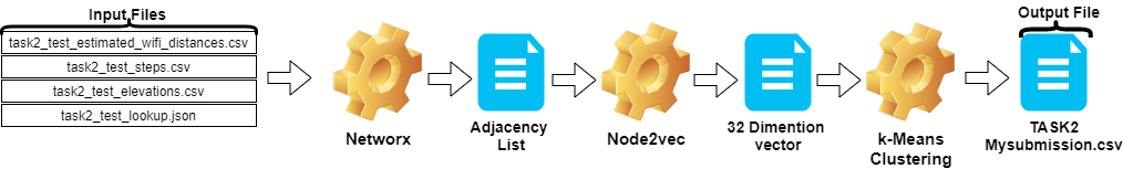
csv_writer . writerows ( random_data )任務2中的步驟可以總結如下:
Node2vec對鄰接列表進行矢量列表。TASK2-Mysubmission.csv )是根據ID的軌跡準備的。這些步驟在下圖中說明。
我們使用Python 3.6.5創建應用程序文件。我們包括了一些其他模塊,這些模塊未包含在比賽開始時給出的示例文件中。這些模塊可以列為:
| molules | 任務 |
|---|---|
| Scikit-Learn | 機器學習和數據準備 |
| node2vec | 網絡的可擴展功能學習 |
| numpy | 數學操作 |
我們從安裝這些模塊作為第一步。
 ## 2.1 Installing modules
!p ip install node2vec
!p ip install scikit - learn
!p ip install numpy 在此步驟中,我們修復了相關的隨機種子以獲得可重複的結果。這樣,我們提供了一個確定性的路徑,在每次運行中都會獲得相同的結果。但是,根據我們的觀察,在不同計算機上獲得的結果可能略有不同(±1%)
 ## 2.2  Setting Random Seeds
seed_value = 0
import os
os . environ [ 'PYTHONHASHSEED' ] = str ( seed_value )
import random
random . seed ( seed_value )
import numpy as np
np . random . seed ( seed_value )在本節中,加載了用於測試數據的文件。
wifi變量從task2_test_estimated_wifi_distances.csv中獲取ID和權重。steps變量從文件task2_test_steps.csv中獲取ID和權重。elevs變量從文件task2_test_elevations.csv中獲取ID。fp_lookup變量從task2_test_lookup.json文件中獲取ID和軌跡。我們不希望使用Task1中獲得的模型重新計算WiFi給出的估計距離的方法,因為我們從該過程中獲得的結果沒有顯著差異。這就是為什麼我們沒有在最終工作中使用task2_test_fingerprints.json文件的原因。
 ## 2.3 Loading the data
import os
import json
import csv
import networkx as nx
from tqdm import tqdm

path_to_data = "task2_for_participants/test"

with open ( os . path . join ( path_to_data , "task2_test_estimated_wifi_distances.csv" )) as f :
    wifi = []
    reader = csv . DictReader ( f )
    for line in tqdm ( reader ):
        wifi . append ([ line [ 'id1' ], line [ 'id2' ], float ( line [ 'estimated_distance' ])])

with open ( os . path . join ( path_to_data , "task2_test_elevations.csv" )) as f :
    elevs = []
    reader = csv . DictReader ( f )
    for line in tqdm ( reader ):
        elevs . append ([ line [ 'id1' ], line [ 'id2' ]])

with open ( os . path . join ( path_to_data , "task2_test_steps.csv" )) as f :
    steps = []
    reader = csv . DictReader ( f )
    for line in tqdm ( reader ):
        steps . append ([ line [ 'id1' ], line [ 'id2' ], float ( line [ 'displacement' ])])

fp_lookup_path = os . path . join ( path_to_data , "task2_test_lookup.json" )

with open ( fp_lookup_path ) as f :
    fp_lookup = json . load ( f )
3773297it [00:19, 191689.25it/s]
2767it [00:00, 52461.27it/s]
139537it [00:00, 180082.01it/s]
創建軌跡圖時,我們將平均距離作為權重。我們為任務2( Task2-IPS-Challenge-2021.ipynb )提供了此過程的示例。我們將結果圖( B )保存為目錄中的鄰接列表(作為my.adjlist )。
 ## 2.3 Generating the Trajectory  graph.
B = nx . Graph ()

# Get all the trajectory ids from the lookup
valid_nodes = set ( fp_lookup . values ())

for node in valid_nodes :
    B . add_node ( node )

# Either add an edge or append the distance to the edge data
for id1 , id2 , dist in tqdm ( wifi ):
    if not B . has_edge ( fp_lookup [ str ( id1 )], fp_lookup [ str ( id2 )]):

        B . add_edge ( fp_lookup [ str ( id1 )],
                   fp_lookup [ str ( id2 )],
                   ty = "w" , weight = [ dist ])
    else :
        B [ fp_lookup [ str ( id1 )]][ fp_lookup [ str ( id2 )]][ 'weight' ]. append ( dist )

# Compute the mean edge weight
for edge in B . edges ( data = True ):
    B [ edge [ 0 ]][ edge [ 1 ]][ 'weight' ] = sum ( B [ edge [ 0 ]][ edge [ 1 ]][ 'weight' ]) / len ( B [ edge [ 0 ]][ edge [ 1 ]][ 'weight' ])

# If you have made a wifi connection between trajectories with an elev, delete the edge
for id1 , id2 in tqdm ( elevs ):
    if B . has_edge ( fp_lookup [ str ( id1 )], fp_lookup [ str ( id2 )]):
        B . remove_edge ( fp_lookup [ str ( id1 )],
                      fp_lookup [ str ( id2 )])

nx . write_adjlist ( B , "my.adjlist" )
100%|████████████████████████████████████████████████████████████████████| 3773297/3773297 [00:27<00:00, 135453.95it/s]
100%|██████████████████████████████████████████████████████████████████████████████████████| 2767/2767 [00:00<?, ?it/s]
在將鄰接列表作為機器學習算法的輸入之前,我們將節點轉換為向量。在我們的工作中,我們將Node2Vec用作嵌入Grover&Leskovec在2016年提出的算法方法的圖表[3]。 Node2Vec是一種半監督算法,用於網絡中的節點的特徵學習。 Node2Vec是基於跳過的技術創建的,該技術是一種NLP方法,該方法是出於分佈結構概念的動機。根據想法,如果在相似上下文中使用的不同單詞可能具有相似的含義,並且它們之間存在明顯的關係。 Skip-gram技術使用中心詞(輸入)來預測鄰居(輸出),而基於給定的窗口大小(中心之後的項目的連續序列)計算周圍環境的概率,換句話說。與NLP方法不同,Node2Vec系統不是帶有線性結構的單詞,而是具有分佈式圖形結構的節點和邊緣。這種多維結構使嵌入式嵌入式複雜且計算昂貴,但是Node2Vec使用負抽樣來優化隨機梯度下降(SGD)來處理它。除此之外,隨機步行方法還用於檢測非線性結構中源節點相鄰節點的樣本。
在我們的研究中,我們首先通過從給定兩個節點的給定距離(權重)的node2VEC建模低維空間中節點關係的矢量表示。然後,我們使用了帶有節點向量的Node2Vec(圖嵌入)的輸出來饋送傳統的K-均值聚類算法。
我們在NOD2VEC中使用的參數可以如下列出:
| 超參數 | 價值 |
|---|---|
| 方面 | 32 |
| walk_length | 15 |
| num_walks | 100 |
| 工人 | 1 |
| 種子 | 0 |
| 窗戶 | 10 |
| min_count | 1 |
| batch_words | 4 |
Node2VEC模型將鄰接列表作為輸入列表,並輸出32尺寸的向量。在此部分中,node.py文件是在Jupyter Notebook中創建並運行的。有兩個原因是,最好在jupyter筆記本電腦單元格中運行外部而不是在外部運行。
Node2vec是一種非常昂貴的方法,如果在Jupyter Notebook中運行,則可能會出現RAM溢出錯誤。在外部創建和運行Node2vec模型避免了此錯誤。下面的單元格創建了名為node.py的文件。該文件創建Node2Vec模型。該模型將鄰接列表( my.adjlist )作為輸入,並創建一個32維向量文件作為輸出( vectors.emb )。
重要的!下面的代碼應在Linux發行版中運行(在Google Colab和Ubuntu中進行了測試)。
 # 2.4 Converting nodes to vectors
# A folder named tmp is created. This folder is essential for the node2vec model to use less RAM.
try :
    if not os . path . exists ( "tmp" ):
        os . makedirs ( "tmp" )
except OSError :
    print ( "The folder could not be created! n Please manually create the " tmp " folder in the directory" )


node = """

# importing related modules

from node2vec import Node2Vec
import networkx as nx

#importing  adjacency list file as B
B = nx.read_adjlist("my.adjlist")

seed_value=0


# Specifying the input and hyperparameters of the node2vec model
node2vec = Node2Vec(B, dimensions=32, walk_length=15, num_walks=100, workers=1,seed=seed_value,temp_folder = './tmp')

#Assigning/specifying random seeds

import os
os.environ['PYTHONHASHSEED']=str(seed_value)

import random
random.seed(seed_value)

import numpy as np
np.random.seed(seed_value)


# creation of the model

model = node2vec.fit(window=10, min_count=1, batch_words=4,seed=seed_value)


# saving the output vector

model.wv.save_word2vec_format("vectors.emb")

# save the model
model.save("vectorMODEL")

"""
f = open ( "node.py" , "w" )
f . write ( node )
f . close ()


! PYTHONHASHSEED = 0 python3 node . py 創建向量文件後,我們讀取此文件( vectors.emb )。該文件由33列組成。第一列是節點號(ID),保留為矢量值。通過按第一列對整個文件進行排序,我們將節點返回其原始順序。然後,我們刪除此ID列,我們將不再使用。因此,我們給出數據的最終形狀。我們的數據已準備好用於機器學習應用程序。
 # 2.4 Reshaping data
vec = np . loadtxt ( "vectors.emb" , skiprows = 1 )
print ( "shape of vector file: " , vec . shape )
print ( vec )
vec = vec [ vec [:, 0 ]. argsort ()];
vec = vec [ 0 : vec . shape [ 0 ], 1 : vec . shape [ 1 ]]
shape of vector file: (11162, 33)
[[ 9.1200000e+03 3.9031842e-01 -4.7147268e-01 ... -5.7490986e-02
1.3059708e-01 -5.4280665e-02]
[ 6.5320000e+03 -3.5591956e-02 -9.8558587e-01 ... -2.7217887e-02
5.6435770e-01 -5.7787680e-01]
[ 5.6580000e+03 3.5879680e-01 -4.7564098e-01 ... -9.7607370e-02
1.5506668e-01 1.1333219e-01]
...
[ 2.7950000e+03 1.1724627e-02 1.0272172e-02 ... -4.5596390e-04
-1.1507459e-02 -7.6738600e-04]
[ 4.3380000e+03 1.2865483e-02 1.2103912e-02 ... 1.6619096e-03
1.3672550e-02 1.4605848e-02]
[ 1.1770000e+03 -1.3707868e-03 1.5238028e-02 ... -5.9994194e-04
-1.2986251e-02 1.3706315e-03]]
Task-2是一個聚類問題。我們需要確定解決此問題的前提是我們應該分為多少個集群。為此,我們嘗試了不同的集群數字,並比較了我們獲得的分數。下圖顯示了簇數和獲得的分數的比較。從該圖可以看出,在5到21個異常的波動之後,簇的數量在5到21之間連續增加,並在21之後穩定。出於這個原因,我們專注於研究中21至23之間的簇數。
 # 2.5 Determine the number of clusters
import numpy as np
import matplotlib . pyplot as plt
import seaborn as sns
import matplotlib
% matplotlib inline
sns . set_style ( "whitegrid" )
agglom = [ 24.69 , 28.14 , 28.14 , 28.14 , 30 , 33.33 , 40.88 , 38.70 , 40 , 40 , 40 , 29.12 , 45.85 , 45.85 , 48.00 , 50.17 , 57.83 , 57.83 , 57.83 ]
plt . figure ( figsize = ( 10 , 5 ))
plt . plot ( range ( 5 , 24 ), agglom )
matplotlib . pyplot . xticks ( range ( 5 , 24 ))
plt . title ( 'Number of clusters and performance relationship' )
plt . xlabel ( 'Number of clusters' )
plt . ylabel ( 'Score' )
plt . show ()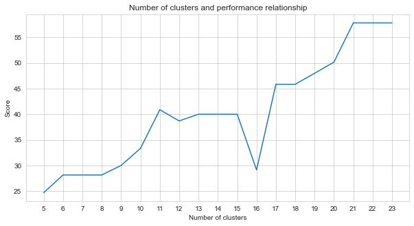
在我們嘗試的無監督的機器學習方法中(例如K-均值,聚集聚類,親和力傳播,平均移位,光譜聚類,DBSCAN,Optics,Optics,birch,Mini Batch k-Meanss),我們使用K -Means取得了最佳效果有23個集群。
K均值是一種聚類算法,是基本的,傳統的無監督機器學習技術之一,它可以使用未標記的數據進行假設,以查找元素或自然組(群集)。集群是將共享特定相似之處分組在一起的一組點(我們的數據中的節點)。 K均值需要質心的目標數,這是指應將數據分為多少組。算法從隨機分配的質心組開始,然後繼續迭代以找到其最佳位置。該算法使用群集將點的正方形總和分配給指定的質心,這是繼續更新和重新定位[4]。在我們的示例中,質心的數量反映了地板的數量。應該注意的是,這不會提供有關地板順序的信息。
下面,已經為23個集群提供了K-均值應用程序。
 # 2.5  Best result
from sklearn import cluster
import time

ML_results = []
k_clusters = 23
algorithms = {}
algorithms [ 'KMeans' ] = cluster . KMeans ( n_clusters = k_clusters , random_state = 10 )
second = time . time ()
for model in algorithms . values ():
    model . fit ( vec )
    ML_results = list ( model . labels_ )
    print ( model , time . time () - second )
KMeans(n_clusters=23, random_state=10) 1.082334280014038
機器學習算法的輸出確定指紋所屬的簇。但是,我們需要的是群集軌跡。因此,這些指紋使用fp_lookup變量將其轉換為其軌跡對應物。該輸出被處理到TASK2-Mysubmission.csv文件中。
 ## 2.6 Submission
result = {}
for ii , i in enumerate ( set ( fp_lookup . values ())):
    result [ i ] = ML_results [ ii ]


ters = {}
for i in result :
    if result [ i ] not in ters :
        ters [ result [ i ]] = []
        ters [ result [ i ]]. append ( i )
    else :
        ters [ result [ i ]]. append ( i )


final_results = []
for i in ters :
    final_results . append ( ters [ i ])


name = "TASK2-Mysubmission.csv"
with open ( name , "w" , newline = '' ) as f :
    csv_writer = csv . writer ( f )
    csv_writer . writerows ( final_results )
print ( name , "file is ready!" )
TASK2-Mysubmission.csv file is ready!
[1] P. Virtanen和Scipy 1.0貢獻者。 Scipy 1.0:Python中科學計算的基本算法。自然方法,17:261--272,2020。
[2] A. Geron,Scikit-Learn,Keras和TensorFlow的動手機器學習:構建智能係統的概念,工具和技術。 O'Reilly Media,2019年
[3] A. Grover,J。Leskovec。 ACM SIGKDD國際知識發現與數據挖掘會議(KDD),2016年。
[4] Jin X.,Han J.(2011)K-均值聚類。在:Sammut C.,Webb GI(EDS)機器學習百科全書。馬薩諸塞州波士頓的施普林格。 https://doi.org/10.1007/978-0-387-30164-8_425


