Sebastian Duchene, Martyna Molak, and Simon Y.W. Ho.
Molecular Ecology, Evolution, and Phylogenetics (MEEP) Laboratory
School of Biological Sciences
University of Sydney
10 June, 2015
partition_data_partitionfinder('drag fasta file with concatenated data here', 'drag partition finder output here')
optim.trees.interactive(folder.parts = 'path to your folder with fasta files and tree topology here')
Implement optimisation of tree distances using the derivative of the BSD distance
Implement parallel version for topology distance
Write tutorial for topology distance clustering
Integrate modelgenerator for model testing
Integrate RaxML for maximum likelihood optimisation of branch lengths and topologies
Estimating evolutionary timescales with multigene data sets is a common exercise in phylogenetic studies. Multigene data sets can be partitioned by gene, codon position, or both. In this tutorial, we refer to “data subsets” as individual genes or any subunit of the multigene data set. The term “partitions” will refer to a group of data subsets.
Although the data subsets can be concatenated and analysed with a single relaxed-clock model, the patterns of among-lineage rate variation can differ between data subsets even when their tree topologies are identical. For instance, the among-lineage rate variation in mitochondrial genes can differ from that of nuclear genes. Therefore, different relaxed-clock models can be assigned to different data subsets in order to improve estimates of evolutionary timescales and statistical fit (see Duchene and Ho., 2014a)
There are a large number of ways in which multigene data sets can be partitioned. A common approach to compare partitioning schemes is to use Bayes factors or likelihood-based criteria for model fit. In most cases, however, it is infeasable to test all possible partitioning schemes, especially with computationally intensive methods of calculating Bayes factors.
ClockstaR estimates the phylogenetic branch lengths of each data subset. The branch-score distance, known as sBSDmin is calculated for every pair of trees as a measure of the difference in their patterns of among-lineage rate variation. These distances are used to infer the best partitioning strategy using the GAP statistic with the PAM clustering algorithm, as implemented in the package cluster (Maechler et al., 2012) (for details of the sBSDmin metric, see Duchene et al., 2014b).
ClockstaR is an R package for phylogenetic molecular clock analyses of multi-gene data sets. It uses the patterns of among lineage rate variation for the different genes to select the clock-partitioning strategy. The method uses a phylogenetic tree distance metric and an unsupervised machine learning algorithm to identify the optimal number of clock-partitoins, and which genes should be analysed under each of the partitons. The partitioning stategy selected in ClocsktaR can be used for subsequent molecular clock analysis with programs such as BEAST, MrBayes, PhyloBayes,and others.
Please follow this link for the original publication.
ClockstaR requires an R installation. It also requires some R dependencies, which can be obtained through R, as explained in bellow.
Please send any requests or questions to Sebastian Duchene (sebastian.duchene[at]sydney.edu.au). Some other software and resources can be found at the Molecular Ecology, Evolution, and Phylogenetics Laboratory at the University of Sydney.
Download a this repository as a zip file and unzip it. The following instructions use the clockstar_example_data folder, which contains some fasta files and a phylogenetic tree in newick format. Open any of these files in a text editor, such as text wrangler. These data were simulated under four pattenrns of evolutionary rate variation. Note that the tree is the tree topology for all genes, or data partitions. To run ClockstaR please format your data similar to the example data in clockstar_example_data.
ClockstaR can be installed directly from GitHub. This requires the devtools package. Type the following code at the R prompt to install all the necessary tools (note you will need internet connection to download the packages directly):.
install.packages("devtools")
library(devtools)
install_github('ClockstaR', 'sebastianduchene')
After downloading and installing, load ClockstaR with the function library.
library(ClockstaR2)To see an example on how the program is run type:
example(ClockstaR2)The rest of this tutorial uses the clockstar_example_data folder
The first step is to obtain the gene trees for each of the alignments. To do this, we use the a tree topology, and optimise the branch lengths using each of the individual gene alignments, in this case A1.fasta through C3.fasta. If you have the gene trees, save then in newick format in a file and got to the next step (running clockstar interactively).
Type the following code in the R prompt and hit enter:
optim.trees.interactive()If you get an error message about installing package phangorn, please use this code and then repeat optim.trees.interactive()
install.packcages("phangorn")ClockstaR will print a the following message:
Please drag a folder with the data subsets and a tree topology. The files should be in FASTA format, and the trees in NEWICKDrag the clockstar_example_data folder to the R console and type enter. Note that the folder should only contain the alingments in FASTA format, and the tree topology in NEWICK. You will see the following message:
What should be the name of the file to save the optimised trees?Type the name of the file for the optimised trees. In this case we will use "example.trees"
example.treesAt this point, ClockstaR will ask whether it should use a separate substitution model for each gene, or use JC in all cases. Since these data were simulated under the JC, we will type "n" and press enter. Type "y" to specify each substitution model separately.
After typing "n" and pressing enter, ClockstaR will start running. It will print the gene trees in the graphics device. If the specified tree was rooted, it may also print a few warnings, which can be safely ignored.
Open the clockstar_example_data folder. You will find a file with name "example.trees", as specified a few steps above. Open example.trees in a text editor. It contains each gene tree and the tree names, accoding to the names of the gene alignments. It should look something like this:
A1.fasta((t1:0.01504695462,(t2:0.00987...
A2.fasta((t1:0.01520523401,(t2:0.01317...
A3.fasta((t1:0.01519309467,(t2:0.01092...
.
.
.
This file with trees will be used for the next step.
For this step it is necessary to have the gene trees in a file, such as that obtained in the previous step.
Open R and load ClockstaR as shown above. Type the following code at the prompt:
clockstar.interactive()ClockstaR will print the following message:
please drag or type in the path to your gene trees file in NEWICK format:Drag the file with the gene trees to the R console. If you followed the previous step, the file will be called example.trees. Type enter.
Depending on the packages you have installed, ClockstaR may ask whether it should run in parallel. This is efficient for large data sets. But for the example data it will not make a big difference, so type "n" if you see this message and then type enter:
Packages foreach and doParallel are available for parallel computation
Should we run ClockstaR in parallel (y / n)? (This is good for large data sets)
Clockstar will now start running. The output on screen should look something like this:
[1] "Calculating sBSDmin distances between all pairs of trees"
[1] "Estimating tree distances"
[1] "estimating distances 1 of 11"
[1] "estimating distances 2 of 11"
[1] "estimating distances 3 of 11"
[1] "estimating distances 4 of 11"
[1] "estimating distances 5 of 11"
.
.
.
After estimating the tree distances (described in the original publication), ClockstaR will print the following message:
"I finished calculating the sBSDmin distances between trees"
The settings for clustering with ClockstaR are:
PAM clustering algorithm
K from 1 to number of data subsets-1
SEmax criterion to select the optimal k
500 bootstrap replicates
 Are these correct? (y/n)
These are the settings for the clustering algorithm. They are appropriate for most data sets, so in this example we can type "y" and then enter.By typing "n" we can change these settings, for more details see Kaufman and Rousseeuw (2009).
ClockstaR will now run the clustering algorithm. At the end it will print the best number of partitions and ask whether the results should be saved in a pdf file:
[1] "ClockstaR has finished running"
[1] "The best number of partitions for your data set is: 3"
Do you wish to save the results in a pdf file?(y/n)
Type "y" then enter.
ClockstaR will then ask for the name of the output files:
What should be the name and path of the output file?For this example type "example_run" and enter, but any name can be used.
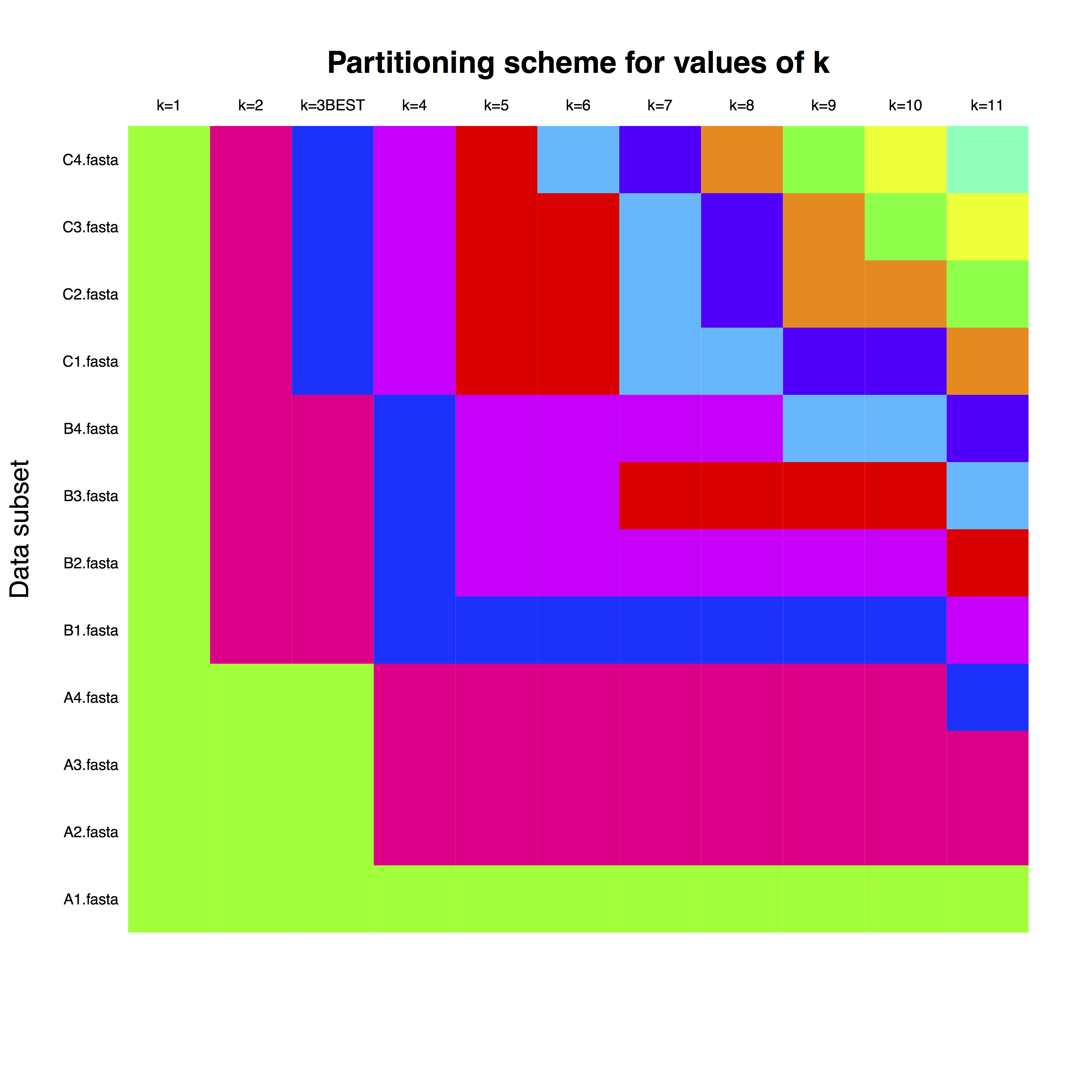
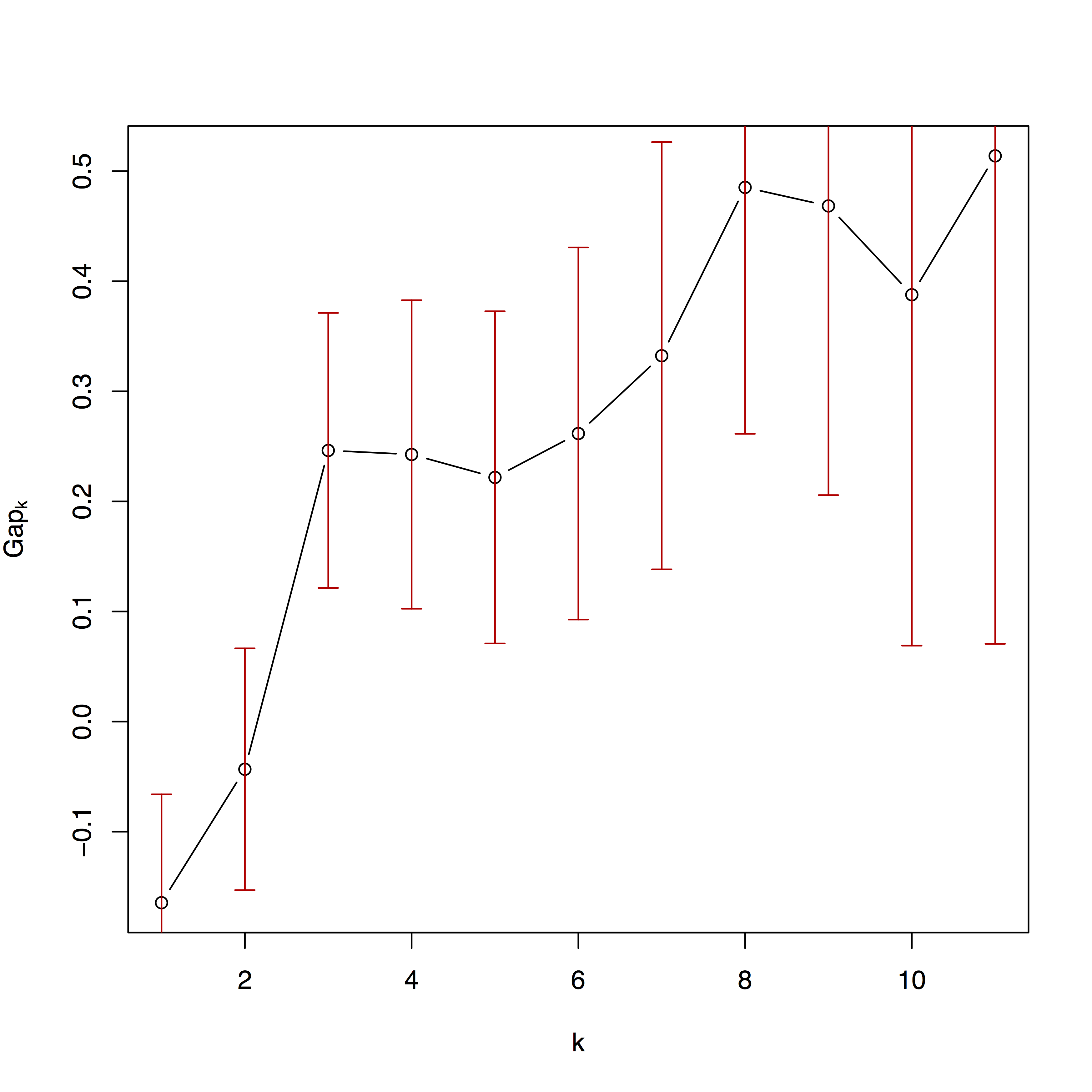
Now open the clockstar_example_data folder and open the two pdf files, example_run_gapstats.pdf and example_run_matrix.pdf.
example_run_matrix is matrix, where rows correspond to each gene, as named in the FASTA files. The columns are the number of partitions, and the colours represent the assignment of each gene to the clock partition. For example, for k=3, which is the best number of partitions, one can use separate clock partitions for genes with letter A, B and C.

The second plot is the fit of the clustering algorithms across different numbers of partitions. More details are available in Kaufman and Rousseeuw (2009) and in the documentation for package cluster.

ClockstaR can be run with other custom settings. Please see the documentation for other details or drop me line for any questions at sebastian.duchene[at]sydney.edy.au.
The logo was designed by Jun Tong
Duchene, S., & Ho, S. Y. (2014a). Using multiple relaxed-clock models to estimate evolutionary timescales from DNA sequence data. Molecular Phylogenetics and Evolution (77): 65-70.
Duchene, S., Molak, M., & Ho, S. Y. (2014b). ClockstaR: choosing the number of relaxed-clock models in molecular phylogenetic analysis. Bioinformatics 30 (7): 1017-1019.
Kaufman, L., & Rousseeuw, P. J. (2009). Finding groups in data: an introduction to cluster analysis (Vol. 344). John Wiley & Sons.