MLE with Normal Distributions - Lab

Introduction

In this lab, we shall put in practice, the mathematical formulas we saw in previous lesson to see how MLE works with normal distributions.

Objectives

You will be able to:

Understand and describe how MLE works with normal distributions
Fit a normal distribution to given data identifying mean and variance
Visually compare the fitted distribution vs. real distribution

Note: *A detailed derivation of all MLE equations with proofs can be seen at this website. *

MLE in Python

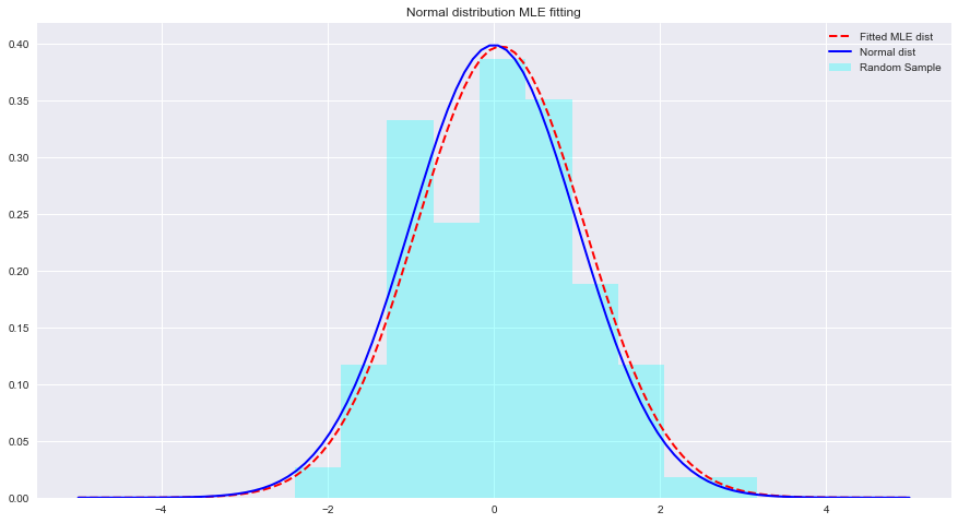
Let's see an example of MLE and distribution fittings with Python below. Here scipy.stats.norm.fit calculates the distribution parameters using Maximum Likelihood Estimation.

Import necessary libraries

from scipy.stats import norm # for generating sample data and fitting distributions
import matplotlib.pyplot as plt
plt.style.use('seaborn')
import numpy as np

Generate an array of 200 random sample from a normal dist with mean 0 and stdv 1

sample = None

Distribution fitting through MLE

- Use `stats.norm.fit(data)` to fit a distribution to above data.

- This returns a list of two parameters : (mean,: parameters[0] and std: parameters[1]) via a MLE approach

param = None

#param[0], param[1]
# (0.08241224761452863, 1.002987490235812)

Calculate the PDF from a) actual data parameters b) fitted parameters with `x = np.linspace(-5,5,100)`

x = np.linspace(-5,5,100)

# Generate the pdf from fitted parameters (fitted distribution)
fitted_pdf = None
# Generate the pdf without fitting (normal distribution non fitted)
normal_pdf = None

Visualize both PDFs

# Your code here

png

#  Your comments/observations

Summary

In this short lab, we looked at Bayesian setting in a Gaussian context i.e. when the underlying random variables are normally distributed. We learned that MLE can estimate the unknown parameters of a normal distribution, by maximizing the likelihood of expected mean. The expected mean comes very close to the mean of a non-fitted normal distribution within that parameter space. We shall move ahead with this understanding towards learning how such estimations are performed in estimating means of a number of classes present in the data distribution using Naive Bayes Classifier.

Expand

Additional Information