vit pytorch
1.9.1

Pytorch에서 단일 변환기 인코더만으로 비전 분류에서 SOTA를 달성하는 간단한 방법인 Vision Transformer를 구현합니다. Yannic Kilcher의 비디오에서 중요성에 대해 자세히 설명합니다. 여기에는 실제로 코딩할 내용이 많지 않지만 모든 사람을 위해 배치하여 주의 혁명을 촉진할 수도 있습니다.
사전 학습된 모델을 사용한 Pytorch 구현에 대해서는 여기에서 Ross Wightman의 저장소를 참조하세요.
공식 Jax 저장소는 여기에 있습니다.
연구 과학자 김준호가 만든 tensorflow2 번역도 여기에 있습니다!
Enrico Shippole의 아마 번역!
$ pip install vit-pytorch import torch
from vit_pytorch import ViT
v = ViT (
image_size = 256 ,
patch_size = 32 ,
num_classes = 1000 ,
dim = 1024 ,
depth = 6 ,
heads = 16 ,
mlp_dim = 2048 ,
dropout = 0.1 ,
emb_dropout = 0.1
)
img = torch . randn ( 1 , 3 , 256 , 256 )
preds = v ( img ) # (1, 1000) image_size : 정수patch_size : 정수image_size patch_size 로 나눌 수 있어야 합니다.n = (image_size // patch_size) ** 2 및 n 16보다 커야 합니다 .num_classes : 정수.dim : 정수.nn.Linear(..., dim) 후 출력 텐서의 마지막 차원.depth : 정수heads : 정수mlp_dim : 정수channels : int, 기본값 3 .dropout : [0, 1] 사이 부동 소수점, 기본값은 0. .emb_dropout : [0, 1] 사이에 부동 소수점, 기본값은 0 .pool : 문자열( cls 토큰 풀링 또는 mean 풀링) 원본 논문의 동일한 저자 중 일부의 업데이트에서는 ViT 더 빠르고 효율적으로 훈련할 수 있도록 단순화할 것을 제안합니다.
이러한 단순화에는 2D 정현파 위치 임베딩, 전역 평균 풀링(CLS 토큰 없음), 드롭아웃 없음, 4096이 아닌 1024의 배치 크기, RandAugment 및 MixUp 확장 사용 등이 포함됩니다. 그들은 또한 끝 부분의 단순한 선형이 원래 MLP 헤드보다 크게 나쁘지 않음을 보여줍니다.
아래와 같이 SimpleViT 를 Import하여 사용할 수 있습니다.
 import torch
from vit_pytorch import SimpleViT

v = SimpleViT (
    image_size = 256 ,
    patch_size = 32 ,
    num_classes = 1000 ,
    dim = 1024 ,
    depth = 6 ,
    heads = 16 ,
    mlp_dim = 2048
)

img = torch . randn ( 1 , 3 , 256 , 256 )

preds = v ( img ) # (1, 1000) 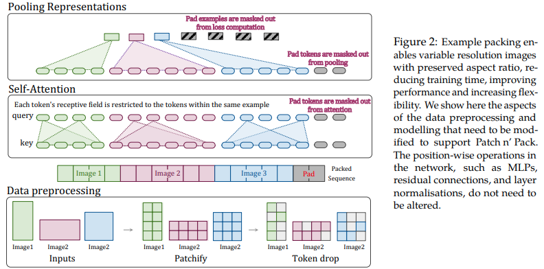
이 논문에서는 다양한 길이의 시퀀스에 대한 주의 및 마스킹의 유연성을 활용하여 단일 배치로 압축된 다중 해상도의 이미지를 훈련하는 것을 제안합니다. 훨씬 더 빠른 훈련과 향상된 정확도를 보여 주며 유일한 비용은 아키텍처 및 데이터 로딩의 추가 복잡성입니다. 인수분해된 2D 위치 인코딩, 토큰 삭제 및 쿼리 키 정규화를 사용합니다.
다음과 같이 사용할 수 있습니다.
 import torch
from vit_pytorch . na_vit import NaViT

v = NaViT (
    image_size = 256 ,
    patch_size = 32 ,
    num_classes = 1000 ,
    dim = 1024 ,
    depth = 6 ,
    heads = 16 ,
    mlp_dim = 2048 ,
    dropout = 0.1 ,
    emb_dropout = 0.1 ,
    token_dropout_prob = 0.1  # token dropout of 10% (keep 90% of tokens)
)

# 5 images of different resolutions - List[List[Tensor]]

# for now, you'll have to correctly place images in same batch element as to not exceed maximum allowed sequence length for self-attention w/ masking

images = [
    [ torch . randn ( 3 , 256 , 256 ), torch . randn ( 3 , 128 , 128 )],
    [ torch . randn ( 3 , 128 , 256 ), torch . randn ( 3 , 256 , 128 )],
    [ torch . randn ( 3 , 64 , 256 )]
]

preds = v ( images ) # (5, 1000) - 5, because 5 images of different resolution above
또는 프레임워크가 특정 최대 길이를 초과하지 않는 가변 길이 시퀀스로 이미지를 자동 그룹화하려는 경우
 images = [
    torch . randn ( 3 , 256 , 256 ),
    torch . randn ( 3 , 128 , 128 ),
    torch . randn ( 3 , 128 , 256 ),
    torch . randn ( 3 , 256 , 128 ),
    torch . randn ( 3 , 64 , 256 )
]

preds = v (
    images ,
    group_images = True ,
    group_max_seq_len = 64
) # (5, 1000)
마지막으로, 중첩된 텐서(많은 마스킹 및 패딩이 모두 생략됨)를 사용하여 NaViT의 특징을 활용하려면 버전 2.5 인지 확인하고 다음과 같이 가져옵니다.
 import torch
from vit_pytorch . na_vit_nested_tensor import NaViT

v = NaViT (
    image_size = 256 ,
    patch_size = 32 ,
    num_classes = 1000 ,
    dim = 1024 ,
    depth = 6 ,
    heads = 16 ,
    mlp_dim = 2048 ,
    dropout = 0. ,
    emb_dropout = 0. ,
    token_dropout_prob = 0.1
)

# 5 images of different resolutions - List[Tensor]

images = [
    torch . randn ( 3 , 256 , 256 ), torch . randn ( 3 , 128 , 128 ),
    torch . randn ( 3 , 128 , 256 ), torch . randn ( 3 , 256 , 128 ),
    torch . randn ( 3 , 64 , 256 )
]

preds = v ( images )

assert preds . shape == ( 5 , 1000 )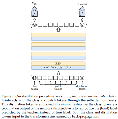
최근 논문에서는 컨벌루션 네트워크에서 비전 변환기로 지식을 증류하기 위해 증류 토큰을 사용하면 작고 효율적인 비전 변환기를 생성할 수 있음을 보여주었습니다. 이 저장소는 쉽게 증류를 수행할 수 있는 수단을 제공합니다.
전. Resnet50(또는 모든 교사)에서 비전 변환기로 증류
 import torch
from torchvision . models import resnet50

from vit_pytorch . distill import DistillableViT , DistillWrapper

teacher = resnet50 ( pretrained = True )

v = DistillableViT (
    image_size = 256 ,
    patch_size = 32 ,
    num_classes = 1000 ,
    dim = 1024 ,
    depth = 6 ,
    heads = 8 ,
    mlp_dim = 2048 ,
    dropout = 0.1 ,
    emb_dropout = 0.1
)

distiller = DistillWrapper (
    student = v ,
    teacher = teacher ,
    temperature = 3 ,           # temperature of distillation
    alpha = 0.5 ,               # trade between main loss and distillation loss
    hard = False               # whether to use soft or hard distillation
)

img = torch . randn ( 2 , 3 , 256 , 256 )
labels = torch . randint ( 0 , 1000 , ( 2 ,))

loss = distiller ( img , labels )
loss . backward ()

# after lots of training above ...

pred = v ( img ) # (2, 1000)
DistillableViT 클래스는 정방향 패스가 처리되는 방식을 제외하고 ViT 와 동일하므로 증류 훈련을 완료한 후 매개변수를 ViT 로 다시 로드할 수 있어야 합니다.
DistillableViT 인스턴스에서 편리한 .to_vit 메서드를 사용하여 ViT 인스턴스를 다시 가져올 수도 있습니다.
 v = v . to_vit ()
type ( v ) # <class 'vit_pytorch.vit_pytorch.ViT'> 이 문서에서는 ViT가 더 깊은 깊이(지난 12개 레이어)에서 주의를 기울이는 데 어려움을 겪고 있음을 지적하고 Re-attention이라는 솔루션으로 소프트맥스 이후 각 헤드의 주의를 혼합할 것을 제안합니다. 결과는 NLP의 Talking Heads 논문과 일치합니다.
다음과 같이 사용할 수 있습니다.
 import torch
from vit_pytorch . deepvit import DeepViT

v = DeepViT (
    image_size = 256 ,
    patch_size = 32 ,
    num_classes = 1000 ,
    dim = 1024 ,
    depth = 6 ,
    heads = 16 ,
    mlp_dim = 2048 ,
    dropout = 0.1 ,
    emb_dropout = 0.1
)

img = torch . randn ( 1 , 3 , 256 , 256 )

preds = v ( img ) # (1, 1000) 또한 이 문서에서는 비전 변환기를 더 깊이 있게 훈련하는 데 어려움이 있음을 지적하고 두 가지 솔루션을 제안합니다. 먼저 잔차 블록의 출력을 채널별로 곱하는 것을 제안합니다. 둘째, 패치가 서로 참석하도록 하고 CLS 토큰이 마지막 몇 레이어의 패치에만 참석하도록 허용할 것을 제안합니다.
또한 Talking Heads를 추가하여 개선 사항을 언급했습니다.
이 구성표를 다음과 같이 사용할 수 있습니다
 import torch
from vit_pytorch . cait import CaiT

v = CaiT (
    image_size = 256 ,
    patch_size = 32 ,
    num_classes = 1000 ,
    dim = 1024 ,
    depth = 12 ,             # depth of transformer for patch to patch attention only
    cls_depth = 2 ,          # depth of cross attention of CLS tokens to patch
    heads = 16 ,
    mlp_dim = 2048 ,
    dropout = 0.1 ,
    emb_dropout = 0.1 ,
    layer_dropout = 0.05    # randomly dropout 5% of the layers
)

img = torch . randn ( 1 , 3 , 256 , 256 )

preds = v ( img ) # (1, 1000) 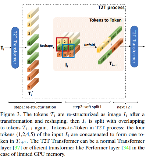
본 논문에서는 위 그림과 같이 첫 번째 몇 개의 레이어가 펼쳐진 이미지 시퀀스를 다운샘플링하여 각 토큰의 이미지 데이터가 겹치도록 제안합니다. 이 ViT 변형을 다음과 같이 사용할 수 있습니다.
 import torch
from vit_pytorch . t2t import T2TViT

v = T2TViT (
    dim = 512 ,
    image_size = 224 ,
    depth = 5 ,
    heads = 8 ,
    mlp_dim = 512 ,
    num_classes = 1000 ,
    t2t_layers = (( 7 , 4 ), ( 3 , 2 ), ( 3 , 2 )) # tuples of the kernel size and stride of each consecutive layers of the initial token to token module
)

img = torch . randn ( 1 , 3 , 224 , 224 )

preds = v ( img ) # (1, 1000) CCT는 패치와 시퀀스 풀링을 수행하는 대신 컨볼루션을 사용하여 컴팩트한 변환기를 제안합니다. 이를 통해 CCT는 높은 정확도와 적은 수의 매개변수를 가질 수 있습니다.
이것을 두 가지 방법으로 사용할 수 있습니다
 import torch
from vit_pytorch . cct import CCT

cct = CCT (
    img_size = ( 224 , 448 ),
    embedding_dim = 384 ,
    n_conv_layers = 2 ,
    kernel_size = 7 ,
    stride = 2 ,
    padding = 3 ,
    pooling_kernel_size = 3 ,
    pooling_stride = 2 ,
    pooling_padding = 1 ,
    num_layers = 14 ,
    num_heads = 6 ,
    mlp_ratio = 3. ,
    num_classes = 1000 ,
    positional_embedding = 'learnable' , # ['sine', 'learnable', 'none']
)

img = torch . randn ( 1 , 3 , 224 , 448 )
pred = cct ( img ) # (1, 1000)
또는 레이어 수, 주의 헤드 수, mlp 비율 및 임베딩 차원을 사전 정의하는 여러 사전 정의된 모델 [2,4,6,7,8,14,16] 중 하나를 사용할 수 있습니다.
 import torch
from vit_pytorch . cct import cct_14

cct = cct_14 (
    img_size = 224 ,
    n_conv_layers = 1 ,
    kernel_size = 7 ,
    stride = 2 ,
    padding = 3 ,
    pooling_kernel_size = 3 ,
    pooling_stride = 2 ,
    pooling_padding = 1 ,
    num_classes = 1000 ,
    positional_embedding = 'learnable' , # ['sine', 'learnable', 'none']
)
공식 저장소에는 사전 학습된 모델 체크포인트에 대한 링크가 포함되어 있습니다.
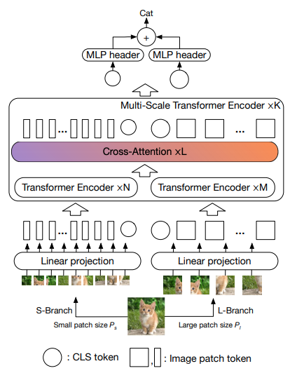
본 논문에서는 서로 다른 규모로 이미지를 처리하는 두 개의 비전 변환기를 사용하고 자주 교차하여 사용하는 것을 제안합니다. 기본 비전 변환기에 대한 개선 사항을 보여줍니다.
 import torch
from vit_pytorch . cross_vit import CrossViT

v = CrossViT (
    image_size = 256 ,
    num_classes = 1000 ,
    depth = 4 ,               # number of multi-scale encoding blocks
    sm_dim = 192 ,            # high res dimension
    sm_patch_size = 16 ,      # high res patch size (should be smaller than lg_patch_size)
    sm_enc_depth = 2 ,        # high res depth
    sm_enc_heads = 8 ,        # high res heads
    sm_enc_mlp_dim = 2048 ,   # high res feedforward dimension
    lg_dim = 384 ,            # low res dimension
    lg_patch_size = 64 ,      # low res patch size
    lg_enc_depth = 3 ,        # low res depth
    lg_enc_heads = 8 ,        # low res heads
    lg_enc_mlp_dim = 2048 ,   # low res feedforward dimensions
    cross_attn_depth = 2 ,    # cross attention rounds
    cross_attn_heads = 8 ,    # cross attention heads
    dropout = 0.1 ,
    emb_dropout = 0.1
)

img = torch . randn ( 1 , 3 , 256 , 256 )

pred = v ( img ) # (1, 1000) 
본 논문에서는 깊이별 컨볼루션을 사용한 풀링 절차를 통해 토큰을 다운샘플링하는 방법을 제안합니다.
 import torch
from vit_pytorch . pit import PiT

v = PiT (
    image_size = 224 ,
    patch_size = 14 ,
    dim = 256 ,
    num_classes = 1000 ,
    depth = ( 3 , 3 , 3 ),     # list of depths, indicating the number of rounds of each stage before a downsample
    heads = 16 ,
    mlp_dim = 2048 ,
    dropout = 0.1 ,
    emb_dropout = 0.1
)

# forward pass now returns predictions and the attention maps

img = torch . randn ( 1 , 3 , 224 , 224 )

preds = v ( img ) # (1, 1000) 
본 논문에서는 (1) 패치 방식 투영 대신 콘볼루셔널 임베딩 (2) 단계별 다운샘플링 (3) 주목의 추가 비선형성 (4) 초기 절대 위치 편향 대신 2D 상대 위치 편향 (5)을 포함한 여러 가지 변경 사항을 제안합니다. ) layernorm 대신에 배치놈을 사용합니다.
공식 저장소
 import torch
from vit_pytorch . levit import LeViT

levit = LeViT (
    image_size = 224 ,
    num_classes = 1000 ,
    stages = 3 ,             # number of stages
    dim = ( 256 , 384 , 512 ),  # dimensions at each stage
    depth = 4 ,              # transformer of depth 4 at each stage
    heads = ( 4 , 6 , 8 ),      # heads at each stage
    mlp_mult = 2 ,
    dropout = 0.1
)

img = torch . randn ( 1 , 3 , 224 , 224 )

levit ( img ) # (1, 1000) 
본 논문에서는 Convolution과 Attention을 혼합하는 방법을 제안합니다. 특히 컨볼루션은 3단계로 이미지/특징 맵을 삽입하고 다운샘플링하는 데 사용됩니다. Depthwise-convoltion은 주의를 끌기 위한 쿼리, 키 및 값을 투영하는 데에도 사용됩니다.
 import torch
from vit_pytorch . cvt import CvT

v = CvT (
    num_classes = 1000 ,
    s1_emb_dim = 64 ,        # stage 1 - dimension
    s1_emb_kernel = 7 ,      # stage 1 - conv kernel
    s1_emb_stride = 4 ,      # stage 1 - conv stride
    s1_proj_kernel = 3 ,     # stage 1 - attention ds-conv kernel size
    s1_kv_proj_stride = 2 ,  # stage 1 - attention key / value projection stride
    s1_heads = 1 ,           # stage 1 - heads
    s1_depth = 1 ,           # stage 1 - depth
    s1_mlp_mult = 4 ,        # stage 1 - feedforward expansion factor
    s2_emb_dim = 192 ,       # stage 2 - (same as above)
    s2_emb_kernel = 3 ,
    s2_emb_stride = 2 ,
    s2_proj_kernel = 3 ,
    s2_kv_proj_stride = 2 ,
    s2_heads = 3 ,
    s2_depth = 2 ,
    s2_mlp_mult = 4 ,
    s3_emb_dim = 384 ,       # stage 3 - (same as above)
    s3_emb_kernel = 3 ,
    s3_emb_stride = 2 ,
    s3_proj_kernel = 3 ,
    s3_kv_proj_stride = 2 ,
    s3_heads = 4 ,
    s3_depth = 10 ,
    s3_mlp_mult = 4 ,
    dropout = 0.
)

img = torch . randn ( 1 , 3 , 224 , 224 )

pred = v ( img ) # (1, 1000) 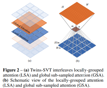
이 문서에서는 이동된 창, CLS 토큰 또는 위치 임베딩의 추가 복잡성 없이 Swin과 동일한 결과를 달성하기 위해 위치 인코딩 생성기(CPVT에서 제안됨) 및 전역 평균 풀링과 함께 로컬 및 전역 관심을 혼합하는 것을 제안합니다.
 import torch
from vit_pytorch . twins_svt import TwinsSVT

model = TwinsSVT (
    num_classes = 1000 ,       # number of output classes
    s1_emb_dim = 64 ,          # stage 1 - patch embedding projected dimension
    s1_patch_size = 4 ,        # stage 1 - patch size for patch embedding
    s1_local_patch_size = 7 ,  # stage 1 - patch size for local attention
    s1_global_k = 7 ,          # stage 1 - global attention key / value reduction factor, defaults to 7 as specified in paper
    s1_depth = 1 ,             # stage 1 - number of transformer blocks (local attn -> ff -> global attn -> ff)
    s2_emb_dim = 128 ,         # stage 2 (same as above)
    s2_patch_size = 2 ,
    s2_local_patch_size = 7 ,
    s2_global_k = 7 ,
    s2_depth = 1 ,
    s3_emb_dim = 256 ,         # stage 3 (same as above)
    s3_patch_size = 2 ,
    s3_local_patch_size = 7 ,
    s3_global_k = 7 ,
    s3_depth = 5 ,
    s4_emb_dim = 512 ,         # stage 4 (same as above)
    s4_patch_size = 2 ,
    s4_local_patch_size = 7 ,
    s4_global_k = 7 ,
    s4_depth = 4 ,
    peg_kernel_size = 3 ,      # positional encoding generator kernel size
    dropout = 0.              # dropout
)

img = torch . randn ( 1 , 3 , 224 , 224 )

pred = model ( img ) # (1, 1000) 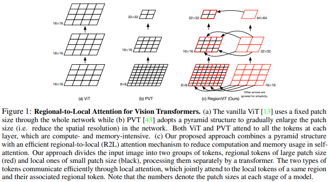
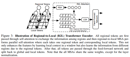
본 논문에서는 기능 맵을 로컬 영역으로 분할하여 로컬 토큰이 서로 참여하는 것을 제안합니다. 각 지역 지역에는 자체 지역 토큰이 있으며, 이 토큰은 모든 지역 토큰과 기타 지역 토큰을 관리합니다.
다음과 같이 사용할 수 있습니다.
 import torch
from vit_pytorch . regionvit import RegionViT

model = RegionViT (
    dim = ( 64 , 128 , 256 , 512 ),      # tuple of size 4, indicating dimension at each stage
    depth = ( 2 , 2 , 8 , 2 ),           # depth of the region to local transformer at each stage
    window_size = 7 ,                # window size, which should be either 7 or 14
    num_classes = 1000 ,             # number of output classes
    tokenize_local_3_conv = False ,  # whether to use a 3 layer convolution to encode the local tokens from the image. the paper uses this for the smaller models, but uses only 1 conv (set to False) for the larger models
    use_peg = False ,                # whether to use positional generating module. they used this for object detection for a boost in performance
)

img = torch . randn ( 1 , 3 , 224 , 224 )

pred = model ( img ) # (1, 1000) 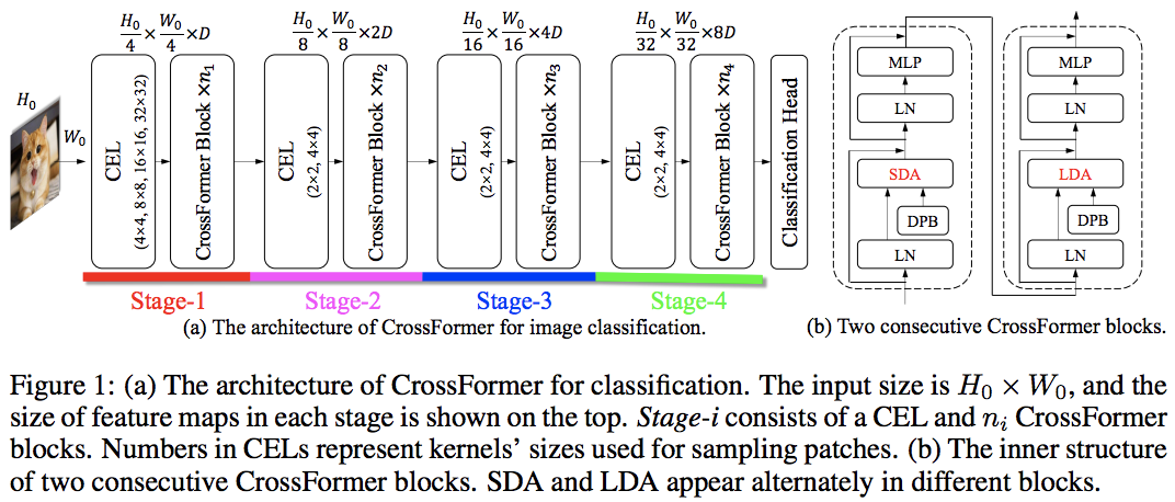
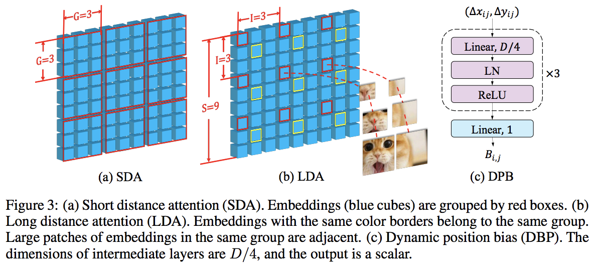
이 논문은 지역 및 글로벌 관심을 번갈아 사용하여 PVT와 Swin을 능가합니다. 전역 주의는 축 주의에 사용되는 방식과 마찬가지로 복잡성을 줄이기 위해 창 차원 전체에 걸쳐 수행됩니다.
또한 모든 비전 변환기를 개선할 수 있는 일반 레이어인 것으로 나타난 크로스 스케일 임베딩 레이어도 있습니다. 또한 네트워크가 더 높은 해상도의 이미지로 일반화될 수 있도록 동적 상대 위치 편향도 공식화되었습니다.
 import torch
from vit_pytorch . crossformer import CrossFormer

model = CrossFormer (
    num_classes = 1000 ,                # number of output classes
    dim = ( 64 , 128 , 256 , 512 ),         # dimension at each stage
    depth = ( 2 , 2 , 8 , 2 ),              # depth of transformer at each stage
    global_window_size = ( 8 , 4 , 2 , 1 ), # global window sizes at each stage
    local_window_size = 7 ,             # local window size (can be customized for each stage, but in paper, held constant at 7 for all stages)
)

img = torch . randn ( 1 , 3 , 224 , 224 )

pred = model ( img ) # (1, 1000) 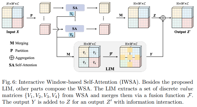
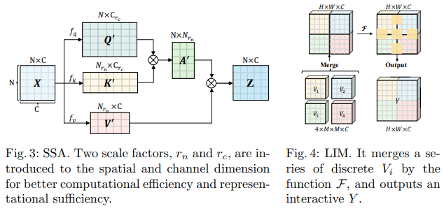
이 Bytedance AI 논문은 SSA(Scalable Self Attention) 및 IWSA(Interactive Windowed Self Attention) 모듈을 제안합니다. SSA는 쿼리와 키의 차원( ssa_dim_key )을 변조하는 동시에 키/값 특성 맵을 일부 요소( reduction_factor )만큼 줄임으로써 초기 단계에 필요한 계산을 완화합니다. IWSA는 다른 비전 변환기 문서와 유사하게 로컬 창 내에서 자기 주의를 수행합니다. 그러나 LIM(Local Interactive Module)이라는 커널 크기 3의 컨볼루션을 통해 전달된 값의 잔차를 추가합니다.
그들은 이 논문에서 이 방식이 Swin Transformer보다 성능이 뛰어나며 Crossformer에 비해 경쟁력 있는 성능을 보여 준다고 주장합니다.
다음과 같이 사용할 수 있습니다. (ex. ScalableViT-S)
 import torch
from vit_pytorch . scalable_vit import ScalableViT

model = ScalableViT (
    num_classes = 1000 ,
    dim = 64 ,                               # starting model dimension. at every stage, dimension is doubled
    heads = ( 2 , 4 , 8 , 16 ),                  # number of attention heads at each stage
    depth = ( 2 , 2 , 20 , 2 ),                  # number of transformer blocks at each stage
    ssa_dim_key = ( 40 , 40 , 40 , 32 ),         # the dimension of the attention keys (and queries) for SSA. in the paper, they represented this as a scale factor on the base dimension per key (ssa_dim_key / dim_key)
    reduction_factor = ( 8 , 4 , 2 , 1 ),        # downsampling of the key / values in SSA. in the paper, this was represented as (reduction_factor ** -2)
    window_size = ( 64 , 32 , None , None ),     # window size of the IWSA at each stage. None means no windowing needed
    dropout = 0.1 ,                          # attention and feedforward dropout
)

img = torch . randn ( 1 , 3 , 256 , 256 )

preds = model ( img ) # (1, 1000) 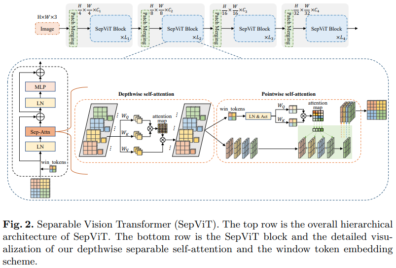
또 다른 Bytedance AI 논문에서는 mobilenet의 깊이별 분리 컨볼루션에서 크게 영감을 받은 것으로 보이는 깊이별 포인트별 self-attention 레이어를 제안합니다. 가장 흥미로운 측면은 위 다이어그램에 표시된 것처럼 깊이별 self-attention 단계의 특징 맵을 점별 self-attention의 값으로 재사용한다는 것입니다.
그룹화된 Attention 레이어는 놀랍지도 참신하지도 않고 저자가 그룹 Self-Attention 레이어의 창 토큰을 어떻게 처리했는지 명확하지 않았기 때문에 나는 이 특정 Self-Attention 레이어에 SepViT 버전만 포함하기로 결정했습니다. 게다가 DSSA 레이어만으로도 Swin을 이길 수 있었던 것 같습니다.
전. SepViT-Lite
 import torch
from vit_pytorch . sep_vit import SepViT

v = SepViT (
    num_classes = 1000 ,
    dim = 32 ,               # dimensions of first stage, which doubles every stage (32, 64, 128, 256) for SepViT-Lite
    dim_head = 32 ,          # attention head dimension
    heads = ( 1 , 2 , 4 , 8 ),   # number of heads per stage
    depth = ( 1 , 2 , 6 , 2 ),   # number of transformer blocks per stage
    window_size = 7 ,        # window size of DSS Attention block
    dropout = 0.1           # dropout
)

img = torch . randn ( 1 , 3 , 224 , 224 )

preds = v ( img ) # (1, 1000) 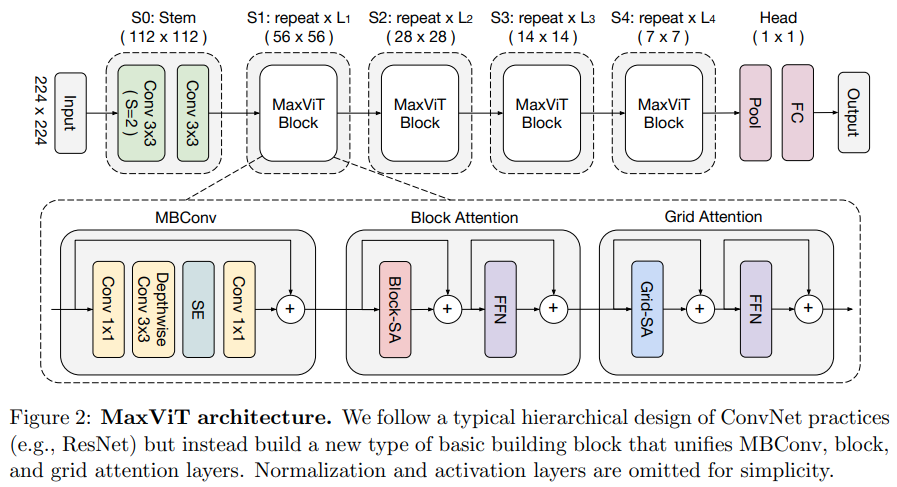
본 논문에서는 컨볼루션 측면에서 MBConv를 사용한 후 블록/그리드 축 희소 어텐션을 사용하는 하이브리드 컨볼루셔널/어텐션 네트워크를 제안합니다.
그들은 또한 이 특정 비전 변환기가 생성 모델(GAN)에 적합하다고 주장합니다.
전. MaxViT-S
 import torch
from vit_pytorch . max_vit import MaxViT

v = MaxViT (
    num_classes = 1000 ,
    dim_conv_stem = 64 ,               # dimension of the convolutional stem, would default to dimension of first layer if not specified
    dim = 96 ,                         # dimension of first layer, doubles every layer
    dim_head = 32 ,                    # dimension of attention heads, kept at 32 in paper
    depth = ( 2 , 2 , 5 , 2 ),             # number of MaxViT blocks per stage, which consists of MBConv, block-like attention, grid-like attention
    window_size = 7 ,                  # window size for block and grids
    mbconv_expansion_rate = 4 ,        # expansion rate of MBConv
    mbconv_shrinkage_rate = 0.25 ,     # shrinkage rate of squeeze-excitation in MBConv
    dropout = 0.1                     # dropout
)

img = torch . randn ( 2 , 3 , 224 , 224 )

preds = v ( img ) # (2, 1000) 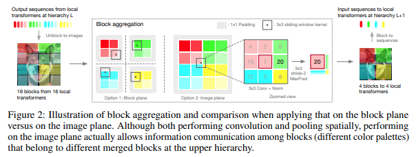
본 논문에서는 계층을 위로 올라갈 때 집계되는 로컬 블록의 토큰 내에서만 주의를 기울여 계층 단계에서 이미지를 처리하기로 결정했습니다. 집계는 이미지 평면에서 수행되며 경계를 넘어 정보를 전달할 수 있도록 컨볼루션과 후속 maxpool을 포함합니다.
다음 코드와 함께 사용할 수 있습니다. (ex. NesT-T)
 import torch
from vit_pytorch . nest import NesT

nest = NesT (
    image_size = 224 ,
    patch_size = 4 ,
    dim = 96 ,
    heads = 3 ,
    num_hierarchies = 3 ,        # number of hierarchies
    block_repeats = ( 2 , 2 , 8 ),  # the number of transformer blocks at each hierarchy, starting from the bottom
    num_classes = 1000
)

img = torch . randn ( 1 , 3 , 224 , 224 )

pred = nest ( img ) # (1, 1000) 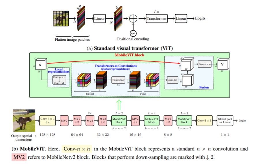
본 논문에서는 모바일 장치를 위한 경량의 범용 비전 변환기인 MobileViT를 소개합니다. MobileViT는 변환기를 사용한 정보의 글로벌 처리에 대한 다른 관점을 제시합니다.
다음 코드(예: mobilevit_xs)와 함께 사용할 수 있습니다.
 import torch
from vit_pytorch . mobile_vit import MobileViT

mbvit_xs = MobileViT (
    image_size = ( 256 , 256 ),
    dims = [ 96 , 120 , 144 ],
    channels = [ 16 , 32 , 48 , 48 , 64 , 64 , 80 , 80 , 96 , 96 , 384 ],
    num_classes = 1000
)

img = torch . randn ( 1 , 3 , 256 , 256 )

pred = mbvit_xs ( img ) # (1, 1000) 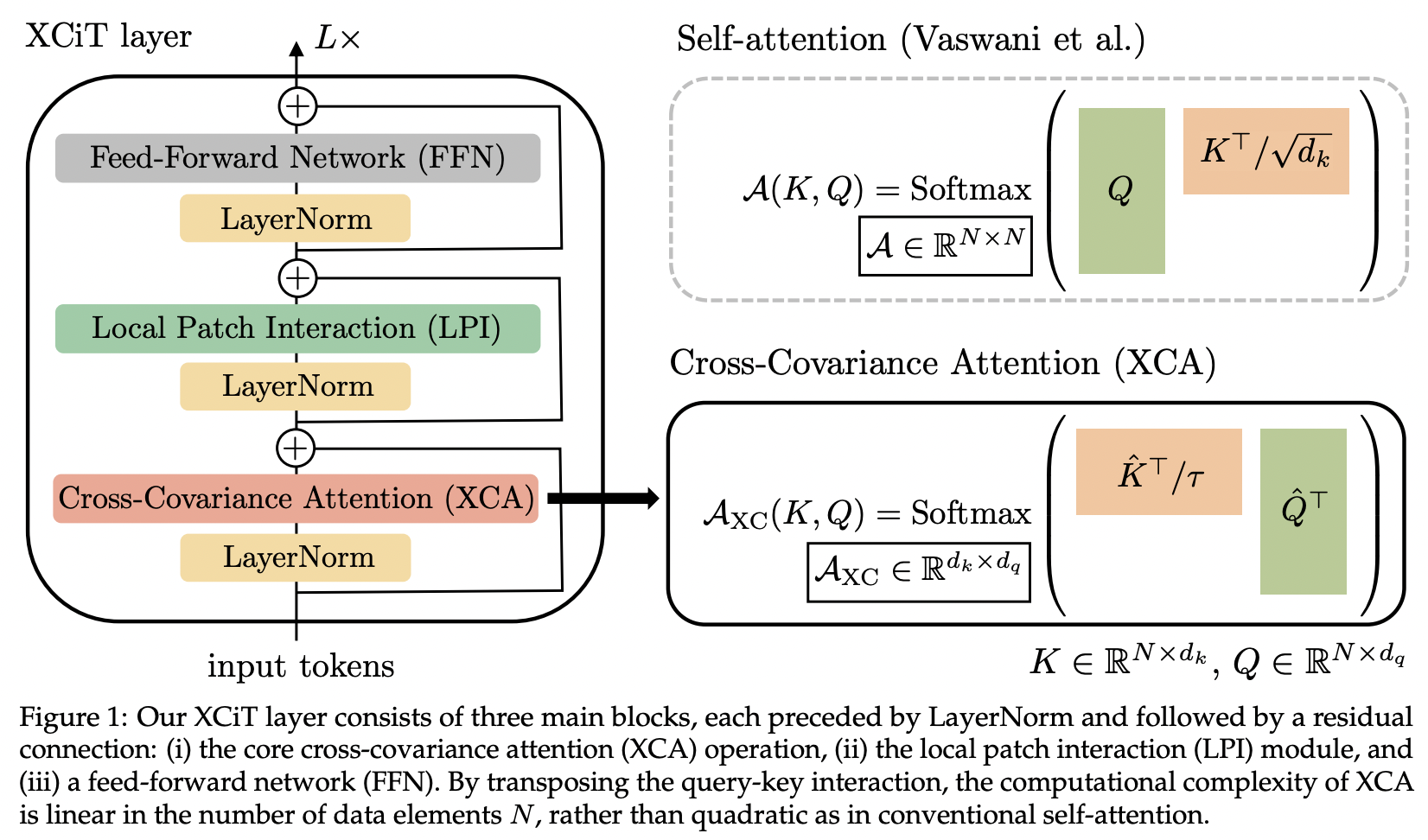
이 논문에서는 교차 공분산 주의(약어로 XCA)를 소개합니다. 공간 차원이 아닌 기능 차원에 걸쳐 주의를 기울이는 것으로 생각할 수 있습니다(또 다른 관점은 동적 1x1 컨볼루션이며 커널은 공간 상관 관계에 의해 정의된 주의 맵입니다).
기술적으로 이는 학습된 온도로 코사인 유사성 주의를 실행하기 전에 단순히 쿼리, 키, 값을 바꾸는 것과 같습니다.
 import torch
from vit_pytorch . xcit import XCiT

v = XCiT (
    image_size = 256 ,
    patch_size = 32 ,
    num_classes = 1000 ,
    dim = 1024 ,
    depth = 12 ,                     # depth of xcit transformer
    cls_depth = 2 ,                  # depth of cross attention of CLS tokens to patch, attention pool at end
    heads = 16 ,
    mlp_dim = 2048 ,
    dropout = 0.1 ,
    emb_dropout = 0.1 ,
    layer_dropout = 0.05 ,           # randomly dropout 5% of the layers
    local_patch_kernel_size = 3     # kernel size of the local patch interaction module (depthwise convs)
)

img = torch . randn ( 1 , 3 , 256 , 256 )

preds = v ( img ) # (1, 1000) 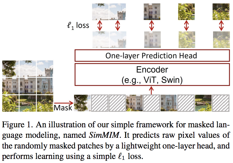
본 논문에서는 마스킹된 토큰을 픽셀 공간으로 선형 투영한 후 마스킹된 패치의 픽셀 값으로 L1 손실을 적용하는 간단한 마스킹된 이미지 모델링(SimMIM) 방식을 제안합니다. 결과는 다른 보다 복잡한 접근 방식에 비해 경쟁력이 있습니다.
이것을 다음과 같이 사용할 수 있습니다
 import torch
from vit_pytorch import ViT
from vit_pytorch . simmim import SimMIM

v = ViT (
    image_size = 256 ,
    patch_size = 32 ,
    num_classes = 1000 ,
    dim = 1024 ,
    depth = 6 ,
    heads = 8 ,
    mlp_dim = 2048
)

mim = SimMIM (
    encoder = v ,
    masking_ratio = 0.5  # they found 50% to yield the best results
)

images = torch . randn ( 8 , 3 , 256 , 256 )

loss = mim ( images )
loss . backward ()

# that's all!
# do the above in a for loop many times with a lot of images and your vision transformer will learn

torch . save ( v . state_dict (), './trained-vit.pt' )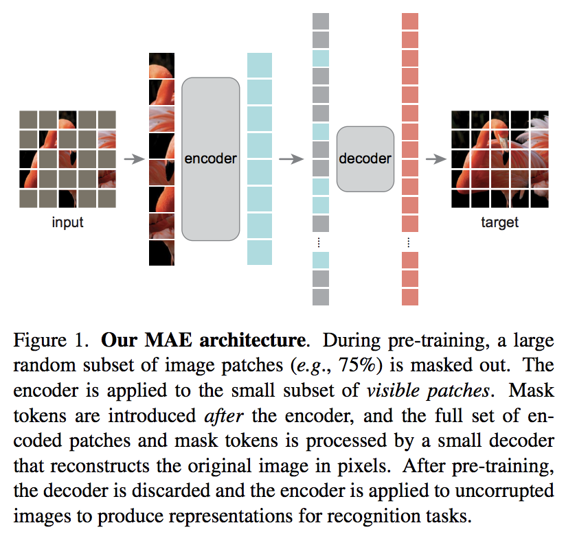
새로운 Kaiming He 논문에서는 비전 변환기가 마스킹되지 않은 패치 세트에 참여하고 더 작은 디코더가 마스킹된 픽셀 값을 재구성하려고 시도하는 간단한 자동 인코더 체계를 제안합니다.
DeepReader 빠른 논문 검토
Letitia와 함께하는 AI 커피브레이크
다음 코드와 함께 사용할 수 있습니다
 import torch
from vit_pytorch import ViT , MAE

v = ViT (
    image_size = 256 ,
    patch_size = 32 ,
    num_classes = 1000 ,
    dim = 1024 ,
    depth = 6 ,
    heads = 8 ,
    mlp_dim = 2048
)

mae = MAE (
    encoder = v ,
    masking_ratio = 0.75 ,   # the paper recommended 75% masked patches
    decoder_dim = 512 ,      # paper showed good results with just 512
    decoder_depth = 6       # anywhere from 1 to 8
)

images = torch . randn ( 8 , 3 , 256 , 256 )

loss = mae ( images )
loss . backward ()

# that's all!
# do the above in a for loop many times with a lot of images and your vision transformer will learn

# save your improved vision transformer
torch . save ( v . state_dict (), './trained-vit.pt' )Zach 덕분에 다음 코드를 사용하여 논문에 제시된 원본 마스크 패치 예측 작업을 사용하여 훈련할 수 있습니다.
 import torch
from vit_pytorch import ViT
from vit_pytorch . mpp import MPP

model = ViT (
    image_size = 256 ,
    patch_size = 32 ,
    num_classes = 1000 ,
    dim = 1024 ,
    depth = 6 ,
    heads = 8 ,
    mlp_dim = 2048 ,
    dropout = 0.1 ,
    emb_dropout = 0.1
)

mpp_trainer = MPP (
    transformer = model ,
    patch_size = 32 ,
    dim = 1024 ,
    mask_prob = 0.15 ,          # probability of using token in masked prediction task
    random_patch_prob = 0.30 ,  # probability of randomly replacing a token being used for mpp
    replace_prob = 0.50 ,       # probability of replacing a token being used for mpp with the mask token
)

opt = torch . optim . Adam ( mpp_trainer . parameters (), lr = 3e-4 )

def sample_unlabelled_images ():
    return torch . FloatTensor ( 20 , 3 , 256 , 256 ). uniform_ ( 0. , 1. )

for _ in range ( 100 ):
    images = sample_unlabelled_images ()
    loss = mpp_trainer ( images )
    opt . zero_grad ()
    loss . backward ()
    opt . step ()

# save your improved network
torch . save ( model . state_dict (), './pretrained-net.pt' )
마스크된 위치 예측 사전 훈련 기준을 소개하는 새로운 논문. 이 전략은 Masked Autoencoder 전략보다 더 효율적이며 비슷한 성능을 갖습니다.
 import torch
from vit_pytorch . mp3 import ViT , MP3

v = ViT (
    num_classes = 1000 ,
    image_size = 256 ,
    patch_size = 8 ,
    dim = 1024 ,
    depth = 6 ,
    heads = 8 ,
    mlp_dim = 2048 ,
    dropout = 0.1 ,
)

mp3 = MP3 (
    vit = v ,
    masking_ratio = 0.75
)

images = torch . randn ( 8 , 3 , 256 , 256 )

loss = mp3 ( images )
loss . backward ()

# that's all!
# do the above in a for loop many times with a lot of images and your vision transformer will learn

# save your improved vision transformer
torch . save ( v . state_dict (), './trained-vit.pt' )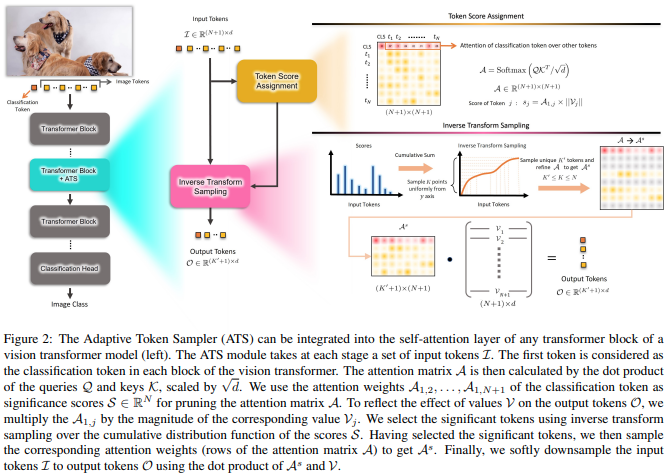
본 논문에서는 서로 다른 계층에서 중요하지 않은 토큰을 폐기하는 수단으로 가치 헤드의 규범에 따라 재평가된 CLS 어텐션 점수를 사용할 것을 제안합니다.
 import torch
from vit_pytorch . ats_vit import ViT

v = ViT (
    image_size = 256 ,
    patch_size = 16 ,
    num_classes = 1000 ,
    dim = 1024 ,
    depth = 6 ,
    max_tokens_per_depth = ( 256 , 128 , 64 , 32 , 16 , 8 ), # a tuple that denotes the maximum number of tokens that any given layer should have. if the layer has greater than this amount, it will undergo adaptive token sampling
    heads = 16 ,
    mlp_dim = 2048 ,
    dropout = 0.1 ,
    emb_dropout = 0.1
)

img = torch . randn ( 4 , 3 , 256 , 256 )

preds = v ( img ) # (4, 1000)

# you can also get a list of the final sampled patch ids
# a value of -1 denotes padding

preds , token_ids = v ( img , return_sampled_token_ids = True ) # (4, 1000), (4, <=8) 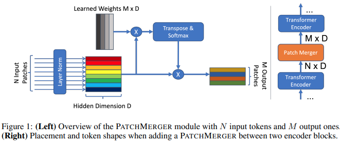
본 논문에서는 성능 저하 없이 비전 변환기의 모든 계층에서 토큰 수를 줄이기 위한 간단한 모듈(Patch Merger)을 제안합니다.
 import torch
from vit_pytorch . vit_with_patch_merger import ViT

v = ViT (
    image_size = 256 ,
    patch_size = 16 ,
    num_classes = 1000 ,
    dim = 1024 ,
    depth = 12 ,
    heads = 8 ,
    patch_merge_layer = 6 ,        # at which transformer layer to do patch merging
    patch_merge_num_tokens = 8 ,   # the output number of tokens from the patch merge
    mlp_dim = 2048 ,
    dropout = 0.1 ,
    emb_dropout = 0.1
)

img = torch . randn ( 4 , 3 , 256 , 256 )

preds = v ( img ) # (4, 1000)
PatchMerger 모듈을 단독으로 사용할 수도 있습니다.
 import torch
from vit_pytorch . vit_with_patch_merger import PatchMerger

merger = PatchMerger (
    dim = 1024 ,
    num_tokens_out = 8   # output number of tokens
)

features = torch . randn ( 4 , 256 , 1024 ) # (batch, num tokens, dimension)

out = merger ( features ) # (4, 8, 1024) 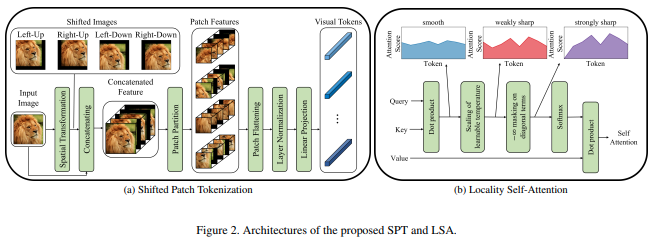
본 논문에서는 이미지를 정규화하고 패치로 분할하기 전에 이미지의 이동을 통합하는 새로운 이미지 패치 기능을 제안합니다. 나는 변속이 일부 다른 변압기 작업에 매우 도움이 된다는 것을 알았으므로 추가 탐색을 위해 이것을 포함하기로 결정했습니다. 또한 학습된 온도를 포함하고 토큰 자체에 대한 관심을 마스킹하는 LSA 도 포함됩니다.
다음과 같이 사용할 수 있습니다:
 import torch
from vit_pytorch . vit_for_small_dataset import ViT

v = ViT (
    image_size = 256 ,
    patch_size = 16 ,
    num_classes = 1000 ,
    dim = 1024 ,
    depth = 6 ,
    heads = 16 ,
    mlp_dim = 2048 ,
    dropout = 0.1 ,
    emb_dropout = 0.1
)

img = torch . randn ( 4 , 3 , 256 , 256 )

preds = v ( img ) # (1, 1000)
이 백서의 SPT 독립형 모듈로 사용할 수도 있습니다.
 import torch
from vit_pytorch . vit_for_small_dataset import SPT

spt = SPT (
    dim = 1024 ,
    patch_size = 16 ,
    channels = 3
)

img = torch . randn ( 4 , 3 , 256 , 256 )

tokens = spt ( img ) # (4, 256, 1024) 많은 분들의 요청에 따라 비디오, 의료 영상 등에 사용할 수 있도록 이 저장소의 아키텍처 중 일부를 3D ViT로 확장하기 시작할 것입니다.
두 개의 추가 하이퍼파라미터((1) frames 수 및 (2) 프레임 차원에 따른 패치 크기)를 전달해야 합니다 frame_patch_size
우선, 3D ViT
 import torch
from vit_pytorch . vit_3d import ViT

v = ViT (
    image_size = 128 ,          # image size
    frames = 16 ,               # number of frames
    image_patch_size = 16 ,     # image patch size
    frame_patch_size = 2 ,      # frame patch size
    num_classes = 1000 ,
    dim = 1024 ,
    depth = 6 ,
    heads = 8 ,
    mlp_dim = 2048 ,
    dropout = 0.1 ,
    emb_dropout = 0.1
)

video = torch . randn ( 4 , 3 , 16 , 128 , 128 ) # (batch, channels, frames, height, width)

preds = v ( video ) # (4, 1000)
3D 단순 ViT
 import torch
from vit_pytorch . simple_vit_3d import SimpleViT

v = SimpleViT (
    image_size = 128 ,          # image size
    frames = 16 ,               # number of frames
    image_patch_size = 16 ,     # image patch size
    frame_patch_size = 2 ,      # frame patch size
    num_classes = 1000 ,
    dim = 1024 ,
    depth = 6 ,
    heads = 8 ,
    mlp_dim = 2048
)

video = torch . randn ( 4 , 3 , 16 , 128 , 128 ) # (batch, channels, frames, height, width)

preds = v ( video ) # (4, 1000)
CCT의 3D 버전
 import torch
from vit_pytorch . cct_3d import CCT

cct = CCT (
    img_size = 224 ,
    num_frames = 8 ,
    embedding_dim = 384 ,
    n_conv_layers = 2 ,
    frame_kernel_size = 3 ,
    kernel_size = 7 ,
    stride = 2 ,
    padding = 3 ,
    pooling_kernel_size = 3 ,
    pooling_stride = 2 ,
    pooling_padding = 1 ,
    num_layers = 14 ,
    num_heads = 6 ,
    mlp_ratio = 3. ,
    num_classes = 1000 ,
    positional_embedding = 'learnable'
)

video = torch . randn ( 1 , 3 , 8 , 224 , 224 ) # (batch, channels, frames, height, width)
pred = cct ( video )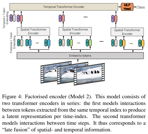
본 논문은 영상의 효율적인 주의를 위한 3가지 유형의 아키텍처를 제안하며, 주요 주제는 공간과 시간에 따른 주의를 고려하는 것입니다. 이 저장소에는 인수분해된 인코더와 인수분해된 self-attention 변형이 포함되어 있습니다. 인수분해된 인코더 변형은 공간 변환기와 시간 변환기가 뒤따르는 것입니다. Factorized self-attention 변형은 공간적 및 시간적 self-attention 레이어가 교대로 있는 시공간 변환기입니다.
 import torch
from vit_pytorch . vivit import ViT

v = ViT (
    image_size = 128 ,          # image size
    frames = 16 ,               # number of frames
    image_patch_size = 16 ,     # image patch size
    frame_patch_size = 2 ,      # frame patch size
    num_classes = 1000 ,
    dim = 1024 ,
    spatial_depth = 6 ,         # depth of the spatial transformer
    temporal_depth = 6 ,        # depth of the temporal transformer
    heads = 8 ,
    mlp_dim = 2048 ,
    variant = 'factorized_encoder' , # or 'factorized_self_attention'
)

video = torch . randn ( 4 , 3 , 16 , 128 , 128 ) # (batch, channels, frames, height, width)

preds = v ( video ) # (4, 1000) 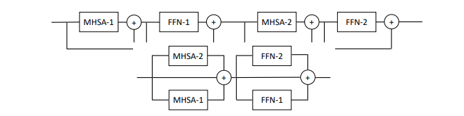
본 논문에서는 레이어당 다중 Attention 및 Feedforward 블록(2블록)을 병렬화하는 것을 제안하며, 성능 손실 없이 훈련하는 것이 더 쉽다고 주장합니다.
다음과 같이 이 변형을 시도해 볼 수 있습니다.
 import torch
from vit_pytorch . parallel_vit import ViT

v = ViT (
    image_size = 256 ,
    patch_size = 16 ,
    num_classes = 1000 ,
    dim = 1024 ,
    depth = 6 ,
    heads = 8 ,
    mlp_dim = 2048 ,
    num_parallel_branches = 2 ,  # in paper, they claimed 2 was optimal
    dropout = 0.1 ,
    emb_dropout = 0.1
)

img = torch . randn ( 4 , 3 , 256 , 256 )

preds = v ( img ) # (4, 1000) 
이 문서에서는 비전 변환기의 각 계층에 학습 가능한 메모리 토큰을 추가하면 미세 조정 결과가 크게 향상될 수 있음을 보여줍니다(학습 가능한 작업별 CLS 토큰 및 어댑터 헤드 외에도).
다음과 같이 특별히 수정된 ViT 와 함께 사용할 수 있습니다.
 import torch
from vit_pytorch . learnable_memory_vit import ViT , Adapter

# normal base ViT

v = ViT (
    image_size = 256 ,
    patch_size = 16 ,
    num_classes = 1000 ,
    dim = 1024 ,
    depth = 6 ,
    heads = 8 ,
    mlp_dim = 2048 ,
    dropout = 0.1 ,
    emb_dropout = 0.1
)

img = torch . randn ( 4 , 3 , 256 , 256 )
logits = v ( img ) # (4, 1000)

# do your usual training with ViT
# ...


# then, to finetune, just pass the ViT into the Adapter class
# you can do this for multiple Adapters, as shown below

adapter1 = Adapter (
    vit = v ,
    num_classes = 2 ,               # number of output classes for this specific task
    num_memories_per_layer = 5     # number of learnable memories per layer, 10 was sufficient in paper
)

logits1 = adapter1 ( img ) # (4, 2) - predict 2 classes off frozen ViT backbone with learnable memories and task specific head

# yet another task to finetune on, this time with 4 classes

adapter2 = Adapter (
    vit = v ,
    num_classes = 4 ,
    num_memories_per_layer = 10
)

logits2 = adapter2 ( img ) # (4, 4) - predict 4 classes off frozen ViT backbone with learnable memories and task specific head 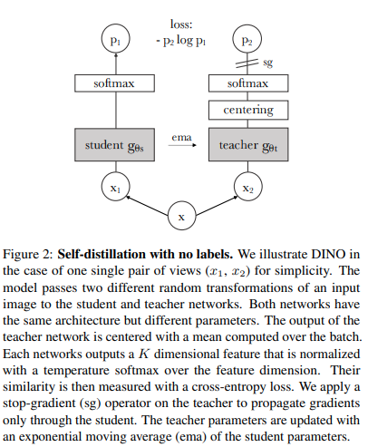
다음 코드를 사용하면 최신 SOTA 자기 지도 학습 기술인 Dino를 사용하여 ViT 훈련할 수 있습니다.
야닉 킬처(Yannic Kilcher) 비디오
 import torch
from vit_pytorch import ViT , Dino

model = ViT (
    image_size = 256 ,
    patch_size = 32 ,
    num_classes = 1000 ,
    dim = 1024 ,
    depth = 6 ,
    heads = 8 ,
    mlp_dim = 2048
)

learner = Dino (
    model ,
    image_size = 256 ,
    hidden_layer = 'to_latent' ,        # hidden layer name or index, from which to extract the embedding
    projection_hidden_size = 256 ,      # projector network hidden dimension
    projection_layers = 4 ,             # number of layers in projection network
    num_classes_K = 65336 ,             # output logits dimensions (referenced as K in paper)
    student_temp = 0.9 ,                # student temperature
    teacher_temp = 0.04 ,               # teacher temperature, needs to be annealed from 0.04 to 0.07 over 30 epochs
    local_upper_crop_scale = 0.4 ,      # upper bound for local crop - 0.4 was recommended in the paper
    global_lower_crop_scale = 0.5 ,     # lower bound for global crop - 0.5 was recommended in the paper
    moving_average_decay = 0.9 ,        # moving average of encoder - paper showed anywhere from 0.9 to 0.999 was ok
    center_moving_average_decay = 0.9 , # moving average of teacher centers - paper showed anywhere from 0.9 to 0.999 was ok
)

opt = torch . optim . Adam ( learner . parameters (), lr = 3e-4 )

def sample_unlabelled_images ():
    return torch . randn ( 20 , 3 , 256 , 256 )

for _ in range ( 100 ):
    images = sample_unlabelled_images ()
    loss = learner ( images )
    opt . zero_grad ()
    loss . backward ()
    opt . step ()
    learner . update_moving_average () # update moving average of teacher encoder and teacher centers

# save your improved network
torch . save ( model . state_dict (), './pretrained-net.pt' )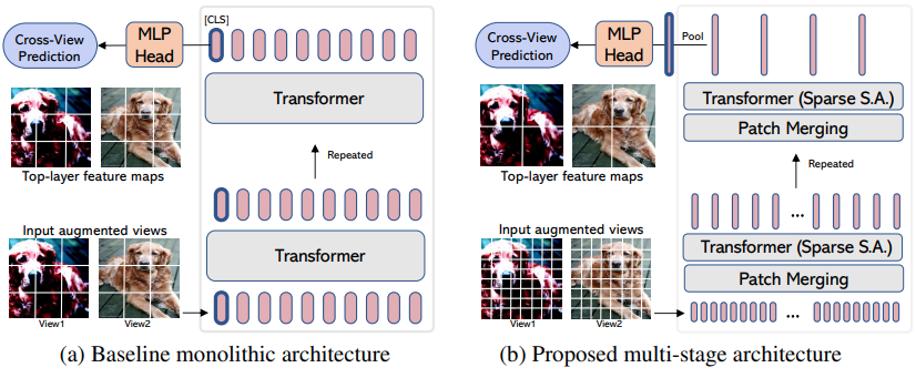
EsViT 는 증강된 뷰 간의 추가 지역 손실을 고려하여 패치 병합/다운샘플링을 통해 효율적인 ViT 를 지원하도록 재설계된 Dino(위)의 변형입니다. 초록을 인용하면 outperforms its supervised counterpart on 17 out of 18 datasets .
새로운 ViT 변종인 것처럼 이름이 붙여졌지만 실제로는 다단계 ViT 훈련하기 위한 전략일 뿐입니다(논문에서는 Swin에 중점을 두었습니다). 아래 예에서는 CvT 와 함께 사용하는 방법을 보여줍니다. 전역 풀링 및 로짓에 대한 투영 직전에 평균이 아닌 풀링된 시각적 표현을 출력하는 효율적인 ViT 내의 레이어 이름으로 hidden_layer 를 설정해야 합니다.
 import torch
from vit_pytorch . cvt import CvT
from vit_pytorch . es_vit import EsViTTrainer

cvt = CvT (
    num_classes = 1000 ,
    s1_emb_dim = 64 ,
    s1_emb_kernel = 7 ,
    s1_emb_stride = 4 ,
    s1_proj_kernel = 3 ,
    s1_kv_proj_stride = 2 ,
    s1_heads = 1 ,
    s1_depth = 1 ,
    s1_mlp_mult = 4 ,
    s2_emb_dim = 192 ,
    s2_emb_kernel = 3 ,
    s2_emb_stride = 2 ,
    s2_proj_kernel = 3 ,
    s2_kv_proj_stride = 2 ,
    s2_heads = 3 ,
    s2_depth = 2 ,
    s2_mlp_mult = 4 ,
    s3_emb_dim = 384 ,
    s3_emb_kernel = 3 ,
    s3_emb_stride = 2 ,
    s3_proj_kernel = 3 ,
    s3_kv_proj_stride = 2 ,
    s3_heads = 4 ,
    s3_depth = 10 ,
    s3_mlp_mult = 4 ,
    dropout = 0.
)

learner = EsViTTrainer (
    cvt ,
    image_size = 256 ,
    hidden_layer = 'layers' ,           # hidden layer name or index, from which to extract the embedding
    projection_hidden_size = 256 ,      # projector network hidden dimension
    projection_layers = 4 ,             # number of layers in projection network
    num_classes_K = 65336 ,             # output logits dimensions (referenced as K in paper)
    student_temp = 0.9 ,                # student temperature
    teacher_temp = 0.04 ,               # teacher temperature, needs to be annealed from 0.04 to 0.07 over 30 epochs
    local_upper_crop_scale = 0.4 ,      # upper bound for local crop - 0.4 was recommended in the paper
    global_lower_crop_scale = 0.5 ,     # lower bound for global crop - 0.5 was recommended in the paper
    moving_average_decay = 0.9 ,        # moving average of encoder - paper showed anywhere from 0.9 to 0.999 was ok
    center_moving_average_decay = 0.9 , # moving average of teacher centers - paper showed anywhere from 0.9 to 0.999 was ok
)

opt = torch . optim . AdamW ( learner . parameters (), lr = 3e-4 )

def sample_unlabelled_images ():
    return torch . randn ( 8 , 3 , 256 , 256 )

for _ in range ( 1000 ):
    images = sample_unlabelled_images ()
    loss = learner ( images )
    opt . zero_grad ()
    loss . backward ()
    opt . step ()
    learner . update_moving_average () # update moving average of teacher encoder and teacher centers

# save your improved network
torch . save ( cvt . state_dict (), './pretrained-net.pt' )연구에 대한 어텐션 가중치(소프트맥스 이후)를 시각화하려면 아래 절차를 따르세요.
 import torch
from vit_pytorch . vit import ViT

v = ViT (
    image_size = 256 ,
    patch_size = 32 ,
    num_classes = 1000 ,
    dim = 1024 ,
    depth = 6 ,
    heads = 16 ,
    mlp_dim = 2048 ,
    dropout = 0.1 ,
    emb_dropout = 0.1
)

# import Recorder and wrap the ViT

from vit_pytorch . recorder import Recorder
v = Recorder ( v )

# forward pass now returns predictions and the attention maps

img = torch . randn ( 1 , 3 , 256 , 256 )
preds , attns = v ( img )

# there is one extra patch due to the CLS token

attns # (1, 6, 16, 65, 65) - (batch x layers x heads x patch x patch)
충분한 데이터를 수집한 후 클래스와 후크를 정리하려면
v = v . eject () # wrapper is discarded and original ViT instance is returned Extractor 래퍼를 사용하여 임베딩에 유사하게 액세스할 수 있습니다.
 import torch
from vit_pytorch . vit import ViT

v = ViT (
    image_size = 256 ,
    patch_size = 32 ,
    num_classes = 1000 ,
    dim = 1024 ,
    depth = 6 ,
    heads = 16 ,
    mlp_dim = 2048 ,
    dropout = 0.1 ,
    emb_dropout = 0.1
)

# import Recorder and wrap the ViT

from vit_pytorch . extractor import Extractor
v = Extractor ( v )

# forward pass now returns predictions and the attention maps

img = torch . randn ( 1 , 3 , 256 , 256 )
logits , embeddings = v ( img )

# there is one extra token due to the CLS token

embeddings # (1, 65, 1024) - (batch x patches x model dim)
또는 '대형' 및 '소형' 스케일에 대해 두 세트의 임베딩을 출력하는 다중 스케일 인코더가 있는 CrossViT 의 경우를 예로 들 수 있습니다.
 import torch
from vit_pytorch . cross_vit import CrossViT

v = CrossViT (
    image_size = 256 ,
    num_classes = 1000 ,
    depth = 4 ,
    sm_dim = 192 ,
    sm_patch_size = 16 ,
    sm_enc_depth = 2 ,
    sm_enc_heads = 8 ,
    sm_enc_mlp_dim = 2048 ,
    lg_dim = 384 ,
    lg_patch_size = 64 ,
    lg_enc_depth = 3 ,
    lg_enc_heads = 8 ,
    lg_enc_mlp_dim = 2048 ,
    cross_attn_depth = 2 ,
    cross_attn_heads = 8 ,
    dropout = 0.1 ,
    emb_dropout = 0.1
)

# wrap the CrossViT

from vit_pytorch . extractor import Extractor
v = Extractor ( v , layer_name = 'multi_scale_encoder' ) # take embedding coming from the output of multi-scale-encoder

# forward pass now returns predictions and the attention maps

img = torch . randn ( 1 , 3 , 256 , 256 )
logits , embeddings = v ( img )

# there is one extra token due to the CLS token

embeddings # ((1, 257, 192), (1, 17, 384)) - (batch x patches x dimension) <- large and small scales respectively 컴퓨터 비전에서 관심이 여전히 2차 비용으로 인해 고통받고 있다고 생각하는 사람들이 있을 수 있습니다. 다행히도 도움이 될 수 있는 새로운 기술이 많이 있습니다. 이 저장소는 자신만의 Sparse Attention Transformer를 플러그인할 수 있는 방법을 제공합니다.
Nystromformer의 예
$ pip install nystrom-attention import torch
from vit_pytorch . efficient import ViT
from nystrom_attention import Nystromformer
efficient_transformer = Nystromformer (
dim = 512 ,
depth = 12 ,
heads = 8 ,
num_landmarks = 256
)
v = ViT (
dim = 512 ,
image_size = 2048 ,
patch_size = 32 ,
num_classes = 1000 ,
transformer = efficient_transformer
)
img = torch . randn ( 1 , 3 , 2048 , 2048 ) # your high resolution picture
v ( img ) # (1, 1000)제가 적극 추천하고 싶은 다른 Sparse Attention 프레임워크는 Routing Transformer 또는 Sinkhorn Transformer입니다.
이 논문은 성명을 발표하기 위해 의도적으로 가장 바닐라적인 관심 네트워크를 사용했습니다. Attention Nets에 대한 최신 개선 사항 중 일부를 사용하려면 이 저장소의 Encoder 사용하십시오.
전.
$ pip install x-transformers import torch
from vit_pytorch . efficient import ViT
from x_transformers import Encoder
v = ViT (
dim = 512 ,
image_size = 224 ,
patch_size = 16 ,
num_classes = 1000 ,
transformer = Encoder (
dim = 512 , # set to be the same as the wrapper
depth = 12 ,
heads = 8 ,
ff_glu = True , # ex. feed forward GLU variant https://arxiv.org/abs/2002.05202
residual_attn = True # ex. residual attention https://arxiv.org/abs/2012.11747
)
)
img = torch . randn ( 1 , 3 , 224 , 224 )
v ( img ) # (1, 1000) 정사각형이 아닌 이미지를 이미 전달할 수 있습니다. 높이와 너비가 image_size 보다 작거나 같고 둘 다 patch_size 로 나눌 수 있는지 확인하면 됩니다.
전.
 import torch
from vit_pytorch import ViT

v = ViT (
    image_size = 256 ,
    patch_size = 32 ,
    num_classes = 1000 ,
    dim = 1024 ,
    depth = 6 ,
    heads = 16 ,
    mlp_dim = 2048 ,
    dropout = 0.1 ,
    emb_dropout = 0.1
)

img = torch . randn ( 1 , 3 , 256 , 128 ) # <-- not a square

preds = v ( img ) # (1, 1000) import torch
from vit_pytorch import ViT
v = ViT (
num_classes = 1000 ,
image_size = ( 256 , 128 ), # image size is a tuple of (height, width)
patch_size = ( 32 , 16 ), # patch size is a tuple of (height, width)
dim = 1024 ,
depth = 6 ,
heads = 16 ,
mlp_dim = 2048 ,
dropout = 0.1 ,
emb_dropout = 0.1
)
img = torch . randn ( 1 , 3 , 256 , 128 )
preds = v ( img )컴퓨터 비전을 접하고 트랜스포머를 처음 접하시나요? 다음은 내 학습을 크게 가속화한 몇 가지 리소스입니다.
일러스트레이트된 트랜스포머 - Jay Alammar
트랜스포머 프롬 스크래치 - 피터 블룸
주석이 달린 변환기 - Harvard NLP
 @article { hassani2021escaping ,
    title   = { Escaping the Big Data Paradigm with Compact Transformers } ,
    author  = { Ali Hassani and Steven Walton and Nikhil Shah and Abulikemu Abuduweili and Jiachen Li and Humphrey Shi } ,
    year    = 2021 ,
    url     = { https://arxiv.org/abs/2104.05704 } ,
    eprint  = { 2104.05704 } ,
    archiveprefix = { arXiv } ,
    primaryclass = { cs.CV }
}
@misc { dosovitskiy2020image ,
title = { An Image is Worth 16x16 Words: Transformers for Image Recognition at Scale } ,
author = { Alexey Dosovitskiy and Lucas Beyer and Alexander Kolesnikov and Dirk Weissenborn and Xiaohua Zhai and Thomas Unterthiner and Mostafa Dehghani and Matthias Minderer and Georg Heigold and Sylvain Gelly and Jakob Uszkoreit and Neil Houlsby } ,
year = { 2020 } ,
eprint = { 2010.11929 } ,
archivePrefix = { arXiv } ,
primaryClass = { cs.CV }
} @misc { touvron2020training ,
title = { Training data-efficient image transformers & distillation through attention } ,
author = { Hugo Touvron and Matthieu Cord and Matthijs Douze and Francisco Massa and Alexandre Sablayrolles and Hervé Jégou } ,
year = { 2020 } ,
eprint = { 2012.12877 } ,
archivePrefix = { arXiv } ,
primaryClass = { cs.CV }
} @misc { yuan2021tokenstotoken ,
title = { Tokens-to-Token ViT: Training Vision Transformers from Scratch on ImageNet } ,
author = { Li Yuan and Yunpeng Chen and Tao Wang and Weihao Yu and Yujun Shi and Francis EH Tay and Jiashi Feng and Shuicheng Yan } ,
year = { 2021 } ,
eprint = { 2101.11986 } ,
archivePrefix = { arXiv } ,
primaryClass = { cs.CV }
} @misc { zhou2021deepvit ,
title = { DeepViT: Towards Deeper Vision Transformer } ,
author = { Daquan Zhou and Bingyi Kang and Xiaojie Jin and Linjie Yang and Xiaochen Lian and Qibin Hou and Jiashi Feng } ,
year = { 2021 } ,
eprint = { 2103.11886 } ,
archivePrefix = { arXiv } ,
primaryClass = { cs.CV }
} @misc { touvron2021going ,
title = { Going deeper with Image Transformers } ,
author = { Hugo Touvron and Matthieu Cord and Alexandre Sablayrolles and Gabriel Synnaeve and Hervé Jégou } ,
year = { 2021 } ,
eprint = { 2103.17239 } ,
archivePrefix = { arXiv } ,
primaryClass = { cs.CV }
} @misc { chen2021crossvit ,
title = { CrossViT: Cross-Attention Multi-Scale Vision Transformer for Image Classification } ,
author = { Chun-Fu Chen and Quanfu Fan and Rameswar Panda } ,
year = { 2021 } ,
eprint = { 2103.14899 } ,
archivePrefix = { arXiv } ,
primaryClass = { cs.CV }
} @misc { wu2021cvt ,
title = { CvT: Introducing Convolutions to Vision Transformers } ,
author = { Haiping Wu and Bin Xiao and Noel Codella and Mengchen Liu and Xiyang Dai and Lu Yuan and Lei Zhang } ,
year = { 2021 } ,
eprint = { 2103.15808 } ,
archivePrefix = { arXiv } ,
primaryClass = { cs.CV }
} @misc { heo2021rethinking ,
title = { Rethinking Spatial Dimensions of Vision Transformers } ,
author = { Byeongho Heo and Sangdoo Yun and Dongyoon Han and Sanghyuk Chun and Junsuk Choe and Seong Joon Oh } ,
year = { 2021 } ,
eprint = { 2103.16302 } ,
archivePrefix = { arXiv } ,
primaryClass = { cs.CV }
} @misc { graham2021levit ,
title = { LeViT: a Vision Transformer in ConvNet's Clothing for Faster Inference } ,
author = { Ben Graham and Alaaeldin El-Nouby and Hugo Touvron and Pierre Stock and Armand Joulin and Hervé Jégou and Matthijs Douze } ,
year = { 2021 } ,
eprint = { 2104.01136 } ,
archivePrefix = { arXiv } ,
primaryClass = { cs.CV }
} @misc { li2021localvit ,
title = { LocalViT: Bringing Locality to Vision Transformers } ,
author = { Yawei Li and Kai Zhang and Jiezhang Cao and Radu Timofte and Luc Van Gool } ,
year = { 2021 } ,
eprint = { 2104.05707 } ,
archivePrefix = { arXiv } ,
primaryClass = { cs.CV }
} @misc { chu2021twins ,
title = { Twins: Revisiting Spatial Attention Design in Vision Transformers } ,
author = { Xiangxiang Chu and Zhi Tian and Yuqing Wang and Bo Zhang and Haibing Ren and Xiaolin Wei and Huaxia Xia and Chunhua Shen } ,
year = { 2021 } ,
eprint = { 2104.13840 } ,
archivePrefix = { arXiv } ,
primaryClass = { cs.CV }
} @misc { su2021roformer ,
title = { RoFormer: Enhanced Transformer with Rotary Position Embedding } ,
author = { Jianlin Su and Yu Lu and Shengfeng Pan and Bo Wen and Yunfeng Liu } ,
year = { 2021 } ,
eprint = { 2104.09864 } ,
archivePrefix = { arXiv } ,
primaryClass = { cs.CL }
} @misc { zhang2021aggregating ,
title = { Aggregating Nested Transformers } ,
author = { Zizhao Zhang and Han Zhang and Long Zhao and Ting Chen and Tomas Pfister } ,
year = { 2021 } ,
eprint = { 2105.12723 } ,
archivePrefix = { arXiv } ,
primaryClass = { cs.CV }
} @misc { chen2021regionvit ,
title = { RegionViT: Regional-to-Local Attention for Vision Transformers } ,
author = { Chun-Fu Chen and Rameswar Panda and Quanfu Fan } ,
year = { 2021 } ,
eprint = { 2106.02689 } ,
archivePrefix = { arXiv } ,
primaryClass = { cs.CV }
} @misc { wang2021crossformer ,
title = { CrossFormer: A Versatile Vision Transformer Hinging on Cross-scale Attention } ,
author = { Wenxiao Wang and Lu Yao and Long Chen and Binbin Lin and Deng Cai and Xiaofei He and Wei Liu } ,
year = { 2021 } ,
eprint = { 2108.00154 } ,
archivePrefix = { arXiv } ,
primaryClass = { cs.CV }
} @misc { caron2021emerging ,
title = { Emerging Properties in Self-Supervised Vision Transformers } ,
author = { Mathilde Caron and Hugo Touvron and Ishan Misra and Hervé Jégou and Julien Mairal and Piotr Bojanowski and Armand Joulin } ,
year = { 2021 } ,
eprint = { 2104.14294 } ,
archivePrefix = { arXiv } ,
primaryClass = { cs.CV }
} @misc { he2021masked ,
title = { Masked Autoencoders Are Scalable Vision Learners } ,
author = { Kaiming He and Xinlei Chen and Saining Xie and Yanghao Li and Piotr Dollár and Ross Girshick } ,
year = { 2021 } ,
eprint = { 2111.06377 } ,
archivePrefix = { arXiv } ,
primaryClass = { cs.CV }
} @misc { xie2021simmim ,
title = { SimMIM: A Simple Framework for Masked Image Modeling } ,
author = { Zhenda Xie and Zheng Zhang and Yue Cao and Yutong Lin and Jianmin Bao and Zhuliang Yao and Qi Dai and Han Hu } ,
year = { 2021 } ,
eprint = { 2111.09886 } ,
archivePrefix = { arXiv } ,
primaryClass = { cs.CV }
} @misc { fayyaz2021ats ,
title = { ATS: Adaptive Token Sampling For Efficient Vision Transformers } ,
author = { Mohsen Fayyaz and Soroush Abbasi Kouhpayegani and Farnoush Rezaei Jafari and Eric Sommerlade and Hamid Reza Vaezi Joze and Hamed Pirsiavash and Juergen Gall } ,
year = { 2021 } ,
eprint = { 2111.15667 } ,
archivePrefix = { arXiv } ,
primaryClass = { cs.CV }
} @misc { mehta2021mobilevit ,
title = { MobileViT: Light-weight, General-purpose, and Mobile-friendly Vision Transformer } ,
author = { Sachin Mehta and Mohammad Rastegari } ,
year = { 2021 } ,
eprint = { 2110.02178 } ,
archivePrefix = { arXiv } ,
primaryClass = { cs.CV }
} @misc { lee2021vision ,
title = { Vision Transformer for Small-Size Datasets } ,
author = { Seung Hoon Lee and Seunghyun Lee and Byung Cheol Song } ,
year = { 2021 } ,
eprint = { 2112.13492 } ,
archivePrefix = { arXiv } ,
primaryClass = { cs.CV }
} @misc { renggli2022learning ,
title = { Learning to Merge Tokens in Vision Transformers } ,
author = { Cedric Renggli and André Susano Pinto and Neil Houlsby and Basil Mustafa and Joan Puigcerver and Carlos Riquelme } ,
year = { 2022 } ,
eprint = { 2202.12015 } ,
archivePrefix = { arXiv } ,
primaryClass = { cs.CV }
} @misc { yang2022scalablevit ,
title = { ScalableViT: Rethinking the Context-oriented Generalization of Vision Transformer } ,
author = { Rui Yang and Hailong Ma and Jie Wu and Yansong Tang and Xuefeng Xiao and Min Zheng and Xiu Li } ,
year = { 2022 } ,
eprint = { 2203.10790 } ,
archivePrefix = { arXiv } ,
primaryClass = { cs.CV }
} @inproceedings { Touvron2022ThreeTE ,
title = { Three things everyone should know about Vision Transformers } ,
author = { Hugo Touvron and Matthieu Cord and Alaaeldin El-Nouby and Jakob Verbeek and Herv'e J'egou } ,
year = { 2022 }
} @inproceedings { Sandler2022FinetuningIT ,
title = { Fine-tuning Image Transformers using Learnable Memory } ,
author = { Mark Sandler and Andrey Zhmoginov and Max Vladymyrov and Andrew Jackson } ,
year = { 2022 }
} @inproceedings { Li2022SepViTSV ,
title = { SepViT: Separable Vision Transformer } ,
author = { Wei Li and Xing Wang and Xin Xia and Jie Wu and Xuefeng Xiao and Minghang Zheng and Shiping Wen } ,
year = { 2022 }
} @inproceedings { Tu2022MaxViTMV ,
title = { MaxViT: Multi-Axis Vision Transformer } ,
author = { Zhengzhong Tu and Hossein Talebi and Han Zhang and Feng Yang and Peyman Milanfar and Alan Conrad Bovik and Yinxiao Li } ,
year = { 2022 }
} @article { Li2021EfficientSV ,
title = { Efficient Self-supervised Vision Transformers for Representation Learning } ,
author = { Chunyuan Li and Jianwei Yang and Pengchuan Zhang and Mei Gao and Bin Xiao and Xiyang Dai and Lu Yuan and Jianfeng Gao } ,
journal = { ArXiv } ,
year = { 2021 } ,
volume = { abs/2106.09785 }
} @misc { Beyer2022BetterPlainViT
title = { Better plain ViT baselines for ImageNet-1k } ,
author = { Beyer, Lucas and Zhai, Xiaohua and Kolesnikov, Alexander } ,
publisher = { arXiv } ,
year = { 2022 }
}
 @article { Arnab2021ViViTAV ,
    title   = { ViViT: A Video Vision Transformer } ,
    author  = { Anurag Arnab and Mostafa Dehghani and Georg Heigold and Chen Sun and Mario Lucic and Cordelia Schmid } ,
    journal = { 2021 IEEE/CVF International Conference on Computer Vision (ICCV) } ,
    year    = { 2021 } ,
    pages   = { 6816-6826 }
}
@article { Liu2022PatchDropoutEV ,
title = { PatchDropout: Economizing Vision Transformers Using Patch Dropout } ,
author = { Yue Liu and Christos Matsoukas and Fredrik Strand and Hossein Azizpour and Kevin Smith } ,
journal = { ArXiv } ,
year = { 2022 } ,
volume = { abs/2208.07220 }
} @misc { https://doi.org/10.48550/arxiv.2302.01327 ,
doi = { 10.48550/ARXIV.2302.01327 } ,
url = { https://arxiv.org/abs/2302.01327 } ,
author = { Kumar, Manoj and Dehghani, Mostafa and Houlsby, Neil } ,
title = { Dual PatchNorm } ,
publisher = { arXiv } ,
year = { 2023 } ,
copyright = { Creative Commons Attribution 4.0 International }
} @inproceedings { Dehghani2023PatchNP ,
title = { Patch n' Pack: NaViT, a Vision Transformer for any Aspect Ratio and Resolution } ,
author = { Mostafa Dehghani and Basil Mustafa and Josip Djolonga and Jonathan Heek and Matthias Minderer and Mathilde Caron and Andreas Steiner and Joan Puigcerver and Robert Geirhos and Ibrahim M. Alabdulmohsin and Avital Oliver and Piotr Padlewski and Alexey A. Gritsenko and Mario Luvci'c and Neil Houlsby } ,
year = { 2023 }
} @misc { vaswani2017attention ,
title = { Attention Is All You Need } ,
author = { Ashish Vaswani and Noam Shazeer and Niki Parmar and Jakob Uszkoreit and Llion Jones and Aidan N. Gomez and Lukasz Kaiser and Illia Polosukhin } ,
year = { 2017 } ,
eprint = { 1706.03762 } ,
archivePrefix = { arXiv } ,
primaryClass = { cs.CL }
} @inproceedings { dao2022flashattention ,
title = { Flash{A}ttention: Fast and Memory-Efficient Exact Attention with {IO}-Awareness } ,
author = { Dao, Tri and Fu, Daniel Y. and Ermon, Stefano and Rudra, Atri and R{'e}, Christopher } ,
booktitle = { Advances in Neural Information Processing Systems } ,
year = { 2022 }
} @inproceedings { Darcet2023VisionTN ,
title = { Vision Transformers Need Registers } ,
author = { Timoth'ee Darcet and Maxime Oquab and Julien Mairal and Piotr Bojanowski } ,
year = { 2023 } ,
url = { https://api.semanticscholar.org/CorpusID:263134283 }
} @inproceedings { ElNouby2021XCiTCI ,
title = { XCiT: Cross-Covariance Image Transformers } ,
author = { Alaaeldin El-Nouby and Hugo Touvron and Mathilde Caron and Piotr Bojanowski and Matthijs Douze and Armand Joulin and Ivan Laptev and Natalia Neverova and Gabriel Synnaeve and Jakob Verbeek and Herv{'e} J{'e}gou } ,
booktitle = { Neural Information Processing Systems } ,
year = { 2021 } ,
url = { https://api.semanticscholar.org/CorpusID:235458262 }
} @inproceedings { Koner2024LookupViTCV ,
title = { LookupViT: Compressing visual information to a limited number of tokens } ,
author = { Rajat Koner and Gagan Jain and Prateek Jain and Volker Tresp and Sujoy Paul } ,
year = { 2024 } ,
url = { https://api.semanticscholar.org/CorpusID:271244592 }
} @article { Bao2022AllAW ,
title = { All are Worth Words: A ViT Backbone for Diffusion Models } ,
author = { Fan Bao and Shen Nie and Kaiwen Xue and Yue Cao and Chongxuan Li and Hang Su and Jun Zhu } ,
journal = { 2023 IEEE/CVF Conference on Computer Vision and Pattern Recognition (CVPR) } ,
year = { 2022 } ,
pages = { 22669-22679 } ,
url = { https://api.semanticscholar.org/CorpusID:253581703 }
} @misc { Rubin2024 ,
author = { Ohad Rubin } ,
url = { https://medium.com/ @ ohadrubin/exploring-weight-decay-in-layer-normalization-challenges-and-a-reparameterization-solution-ad4d12c24950 }
} @inproceedings { Loshchilov2024nGPTNT ,
title = { nGPT: Normalized Transformer with Representation Learning on the Hypersphere } ,
author = { Ilya Loshchilov and Cheng-Ping Hsieh and Simeng Sun and Boris Ginsburg } ,
year = { 2024 } ,
url = { https://api.semanticscholar.org/CorpusID:273026160 }
} @inproceedings { Liu2017DeepHL ,
title = { Deep Hyperspherical Learning } ,
author = { Weiyang Liu and Yanming Zhang and Xingguo Li and Zhen Liu and Bo Dai and Tuo Zhao and Le Song } ,
booktitle = { Neural Information Processing Systems } ,
year = { 2017 } ,
url = { https://api.semanticscholar.org/CorpusID:5104558 }
} @inproceedings { Zhou2024ValueRL ,
title = { Value Residual Learning For Alleviating Attention Concentration In Transformers } ,
author = { Zhanchao Zhou and Tianyi Wu and Zhiyun Jiang and Zhenzhong Lan } ,
year = { 2024 } ,
url = { https://api.semanticscholar.org/CorpusID:273532030 }
} @article { Zhu2024HyperConnections ,
title = { Hyper-Connections } ,
author = { Defa Zhu and Hongzhi Huang and Zihao Huang and Yutao Zeng and Yunyao Mao and Banggu Wu and Qiyang Min and Xun Zhou } ,
journal = { ArXiv } ,
year = { 2024 } ,
volume = { abs/2409.19606 } ,
url = { https://api.semanticscholar.org/CorpusID:272987528 }
}나는 개들이 인간에게 그러하듯이 우리가 로봇에게 다가가는 시대를 상상하며 기계를 응원합니다. — 클로드 섀넌


