alphafold2
v0.4.32
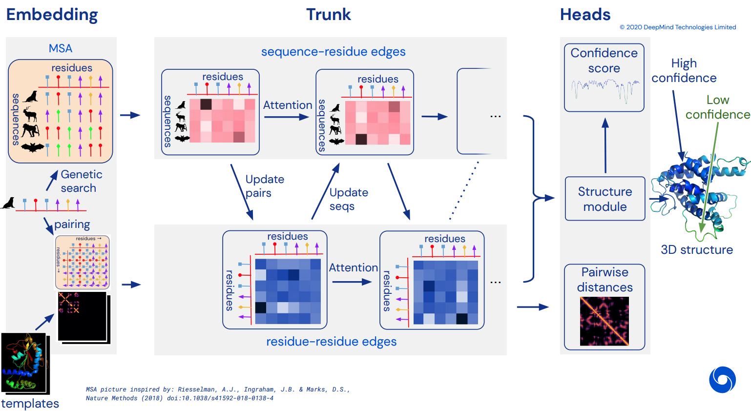
ในที่สุดก็กลายเป็นการใช้งาน Pytorch อย่างไม่เป็นทางการของ Alphafold2 ซึ่งเป็นเครือข่ายความสนใจอันน่าทึ่งที่แก้ไข CASP14 จะทยอยนำมาใช้เมื่อมีการเปิดเผยรายละเอียดสถาปัตยกรรมเพิ่มเติม
เมื่อสิ่งนี้ถูกจำลองขึ้น ฉันตั้งใจที่จะพับลำดับกรดอะมิโนที่มีอยู่ทั้งหมดออกไปในซิลิโก และปล่อยมันเป็นกระแสทางวิชาการ เพื่อเผยแพร่ทางวิทยาศาสตร์ต่อไป หากคุณสนใจที่จะจำลองแบบ โปรดแวะมาที่ #alphafold ที่ช่องทาง Discord นี้
อัปเดต: Deepmind ได้โอเพ่นซอร์สรหัสอย่างเป็นทางการใน Jax พร้อมด้วยน้ำหนัก ! ตอนนี้พื้นที่เก็บข้อมูลนี้จะมุ่งเน้นไปที่การแปลแบบ pytorch แบบตรงพร้อมการปรับปรุงบางอย่างในการเข้ารหัสตำแหน่ง
วิดีโอ ArxivInsights
$ pip install alphafold2-pytorchlhatsk ได้รายงานการฝึกอบรม trunk ที่ดัดแปลงของที่เก็บนี้ โดยใช้การตั้งค่าเดียวกันกับ trRosetta พร้อมผลลัพธ์ที่แข่งขันได้
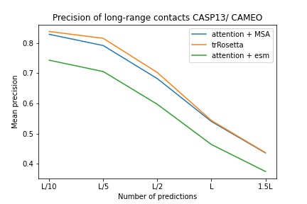
blue used the the trRosetta input (MSA -> potts -> axial attention), green used the ESM embedding (only sequence) -> tiling -> axial attention - lhatsk
การทำนายไดสโตแกรม เช่น Alphafold-1 แต่ด้วยความเอาใจใส่
 import torch
from alphafold2_pytorch import Alphafold2

model = Alphafold2 (
    dim = 256 ,
    depth = 2 ,
    heads = 8 ,
    dim_head = 64 ,
    reversible = False  # set this to True for fully reversible self / cross attention for the trunk
). cuda ()

seq = torch . randint ( 0 , 21 , ( 1 , 128 )). cuda ()      # AA length of 128
msa = torch . randint ( 0 , 21 , ( 1 , 5 , 120 )). cuda ()   # MSA doesn't have to be the same length as primary sequence
mask = torch . ones_like ( seq ). bool (). cuda ()
msa_mask = torch . ones_like ( msa ). bool (). cuda ()

distogram = model (
    seq ,
    msa ,
    mask = mask ,
    msa_mask = msa_mask
) # (1, 128, 128, 37)
คุณยังสามารถเปิดการทำนายสำหรับมุมได้ โดยส่งค่า predict_angles = True ใน init ตัวอย่างด้านล่างจะเทียบเท่ากับ trRosetta แต่เป็นการเอาใจใส่ตนเอง/ข้าม
 import torch
from alphafold2_pytorch import Alphafold2

model = Alphafold2 (
    dim = 256 ,
    depth = 2 ,
    heads = 8 ,
    dim_head = 64 ,
    predict_angles = True   # set this to True
). cuda ()

seq = torch . randint ( 0 , 21 , ( 1 , 128 )). cuda ()
msa = torch . randint ( 0 , 21 , ( 1 , 5 , 120 )). cuda ()
mask = torch . ones_like ( seq ). bool (). cuda ()
msa_mask = torch . ones_like ( msa ). bool (). cuda ()

distogram , theta , phi , omega = model (
    seq ,
    msa ,
    mask = mask ,
    msa_mask = msa_mask
)

# distogram - (1, 128, 128, 37),
# theta     - (1, 128, 128, 25),
# phi       - (1, 128, 128, 13),
# omega - (1, 128, 128, 25) บทความล่าสุดของ Fabian แนะนำให้ป้อนพิกัดกลับเข้าไปใน SE3 Transformer ซ้ำๆ ซึ่งอาจใช้ร่วมกันโดยใช้น้ำหนักร่วมกัน ฉันได้ตัดสินใจที่จะดำเนินการตามแนวคิดนี้ แม้ว่าจะยังคงอยู่ในอากาศว่าวิธีการทำงานจริงเป็นอย่างไร
คุณยังสามารถใช้ E(n)-Transformer หรือ EGNN สำหรับการปรับแต่งโครงสร้างได้
อัปเดต: ห้องทดลองของ Baker ได้แสดงให้เห็นว่าสถาปัตยกรรมแบบ end-to-end จากลำดับและการฝัง MSA ไปจนถึง SE3 Transformers สามารถทำให้ trRosetta ดีที่สุดและปิดช่องว่างกับ Alphafold2 เราจะใช้ Graph Transformer ซึ่งทำหน้าที่ในการฝัง trunk เพื่อสร้างชุดพิกัดเริ่มต้นที่จะส่งไปยังเครือข่ายที่เทียบเท่า (สิ่งนี้ได้รับการยืนยันเพิ่มเติมโดย Costa และคณะในงานของพวกเขาโดยล้อเล่นพิกัด 3 มิติจากการฝัง MSA Transformer ในกระดาษก่อนห้องปฏิบัติการของ Baker)
 import torch
from alphafold2_pytorch import Alphafold2

model = Alphafold2 (
    dim = 256 ,
    depth = 2 ,
    heads = 8 ,
    dim_head = 64 ,
    predict_coords = True ,
    structure_module_type = 'se3' ,          # use SE3 Transformer - if set to False, will use E(n)-Transformer, Victor and Max Welling's new paper
    structure_module_dim = 4 ,               # se3 transformer dimension
    structure_module_depth = 1 ,             # depth
    structure_module_heads = 1 ,             # heads
    structure_module_dim_head = 16 ,         # dimension of heads
    structure_module_refinement_iters = 2 ,  # number of equivariant coordinate refinement iterations
    structure_num_global_nodes = 1          # number of global nodes for the structure module, only works with SE3 transformer
). cuda ()

seq = torch . randint ( 0 , 21 , ( 2 , 64 )). cuda ()
msa = torch . randint ( 0 , 21 , ( 2 , 5 , 60 )). cuda ()
mask = torch . ones_like ( seq ). bool (). cuda ()
msa_mask = torch . ones_like ( msa ). bool (). cuda ()

coords = model (
    seq ,
    msa ,
    mask = mask ,
    msa_mask = msa_mask
) # (2, 64 * 3, 3) <-- 3 atoms per residue สมมติฐานพื้นฐานคือลำตัวทำงานในระดับสารตกค้าง จากนั้นประกอบขึ้นเป็นระดับอะตอมสำหรับโมดูลโครงสร้าง ไม่ว่าจะเป็นหม้อแปลง SE3, E(n)-หม้อแปลงไฟฟ้า หรือ EGNN ที่ทำการปรับแต่ง ไลบรารีนี้มีค่าเริ่มต้นอยู่ที่ 3 อะตอมของแกนหลัก (C, Ca, N) แต่คุณสามารถกำหนดค่าให้รวมอะตอมอื่นๆ ที่คุณต้องการได้ รวมถึง Cb และ sidechains
 import torch
from alphafold2_pytorch import Alphafold2

model = Alphafold2 (
    dim = 256 ,
    depth = 2 ,
    heads = 8 ,
    dim_head = 64 ,
    predict_coords = True ,
    atoms = 'backbone-with-cbeta'
). cuda ()

seq = torch . randint ( 0 , 21 , ( 2 , 64 )). cuda ()
msa = torch . randint ( 0 , 21 , ( 2 , 5 , 60 )). cuda ()
mask = torch . ones_like ( seq ). bool (). cuda ()
msa_mask = torch . ones_like ( msa ). bool (). cuda ()

coords = model (
    seq ,
    msa ,
    mask = mask ,
    msa_mask = msa_mask
) # (2, 64 * 4, 3)  <-- 4 atoms per residue (C, Ca, N, Cb)
ตัวเลือกที่ถูกต้องสำหรับ atoms ได้แก่ :
backbone - 3 อะตอมของกระดูกสันหลัง (C, Ca, N) [ค่าเริ่มต้น]backbone-with-cbeta - 3 อะตอมของกระดูกสันหลังและ C เบต้าbackbone-with-oxygen - 3 อะตอมของกระดูกสันหลังและออกซิเจนจากคาร์บอกซิลbackbone-with-cbeta-and-oxygen - 3 อะตอมของกระดูกสันหลังที่มี C เบต้าและออกซิเจนall - backbone และอะตอมอื่นๆ ทั้งหมดจาก sidechainคุณยังสามารถส่งผ่านเทนเซอร์ของรูปร่าง (14,) เพื่อกำหนดอะตอมที่คุณต้องการรวมไว้ด้วย
อดีต.
atoms = torch . tensor ([ 1 , 1 , 1 , 1 , 1 , 1 , 0 , 1 , 0 , 0 , 0 , 0 , 0 , 1 ])พื้นที่เก็บข้อมูลนี้นำเสนอการเสริมเครือข่ายอย่างง่ายดายด้วยการฝังที่ได้รับการฝึกอบรมล่วงหน้าจาก Facebook AI ประกอบด้วยกระดาษห่อสำหรับหม้อแปลง ESM, MSA หรือหม้อแปลงโปรตีนที่ผ่านการฝึกอบรมมาแล้ว
มีข้อกำหนดเบื้องต้นบางประการ คุณจะต้องตรวจสอบให้แน่ใจว่าคุณได้ติดตั้งไลบรารี่เอเพ็กซ์ของ Nvidia เนื่องจากหม้อแปลงที่ได้รับการฝึกอบรมจะใช้การดำเนินการแบบหลอมละลายบางอย่าง
หรือคุณสามารถลองใช้สคริปต์ด้านล่าง
git clone https://github.com/NVIDIA/apex
cd apex
pip install -v --disable-pip-version-check --no-cache-dir --global-option= " --cpp_ext " --global-option= " --cuda_ext " ./
ถัดไป คุณเพียงแค่ต้องนำเข้าและรวมอินสแตนซ์ Alphafold2 ของคุณด้วย ESMEmbedWrapper , MSAEmbedWrapper หรือ ProtTranEmbedWrapper และมันจะดูแลการฝังทั้งลำดับและการจัดแนวหลายลำดับให้คุณ (และฉายภาพไปยังมิติข้อมูลตามที่ระบุไว้ใน แบบอย่าง). ไม่จำเป็นต้องเปลี่ยนแปลงอะไรนอกจากการเพิ่มกระดาษห่อ
 import torch
from alphafold2_pytorch import Alphafold2
from alphafold2_pytorch . embeds import MSAEmbedWrapper

alphafold2 = Alphafold2 (
    dim = 256 ,
    depth = 2 ,
    heads = 8 ,
    dim_head = 64
)

model = MSAEmbedWrapper (
    alphafold2 = alphafold2
). cuda ()

seq = torch . randint ( 0 , 21 , ( 2 , 16 )). cuda ()
mask = torch . ones_like ( seq ). bool (). cuda ()

msa = torch . randint ( 0 , 21 , ( 2 , 5 , 16 )). cuda ()
msa_mask = torch . ones_like ( msa ). bool (). cuda ()

distogram = model (
    seq ,
    msa ,
    mask = mask ,
    msa_mask = msa_mask
)
ตามค่าเริ่มต้น แม้ว่า wrapper จะจัดเตรียมลำดับและการฝัง MSA ให้กับ Trunk แต่จะถูกรวมเข้ากับการฝังโทเค็นตามปกติ หากคุณต้องการฝึก Alphafold2 โดยไม่มีการฝังโทเค็น (อาศัยการฝังที่ฝึกไว้ล่วงหน้าเท่านั้น) คุณจะต้องตั้ง disable_token_embed เป็น True ใน Alphafold2 init
 alphafold2 = Alphafold2 (
    dim = 256 ,
    depth = 2 ,
    heads = 8 ,
    dim_head = 64 ,
    disable_token_embed = True
) บทความของ Jinbo Xu แนะนำว่าไม่จำเป็นต้องแยกระยะทาง และสามารถทำนายค่าเฉลี่ยและส่วนเบี่ยงเบนมาตรฐานได้โดยตรงแทน คุณสามารถใช้สิ่งนี้ได้โดยเปิดแฟล็กการคาดการณ์หนึ่งค่า predict_real_value_distances ในกรณีนี้ การทำนายระยะทางที่ส่งคืนจะมีมิติเป็น 2 สำหรับค่าเฉลี่ยและส่วนเบี่ยงเบนมาตรฐานตามลำดับ
หากเปิด predict_coords ไว้ด้วย MDS จะยอมรับการคาดคะเนค่าเฉลี่ยและส่วนเบี่ยงเบนมาตรฐานโดยตรง โดยไม่ต้องคำนวณค่านั้นจากถังไดสโตแกรม
 import torch
from alphafold2_pytorch import Alphafold2

model = Alphafold2 (
    dim = 256 ,
    depth = 2 ,
    heads = 8 ,
    dim_head = 64 ,
    predict_coords = True ,
    predict_real_value_distances = True ,      # set this to True
    structure_module_type = 'se3' ,
    structure_module_dim = 4 ,
    structure_module_depth = 1 ,
    structure_module_heads = 1 ,
    structure_module_dim_head = 16 ,
    structure_module_refinement_iters = 2
). cuda ()

seq = torch . randint ( 0 , 21 , ( 2 , 64 )). cuda ()
msa = torch . randint ( 0 , 21 , ( 2 , 5 , 60 )). cuda ()
mask = torch . ones_like ( seq ). bool (). cuda ()
msa_mask = torch . ones_like ( msa ). bool (). cuda ()

coords = model (
    seq ,
    msa ,
    mask = mask ,
    msa_mask = msa_mask
) # (2, 64 * 3, 3) <-- 3 atoms per residue คุณสามารถเพิ่มบล็อกแบบหมุนวนสำหรับทั้งลำดับหลักและ MSA ได้โดยเพียงแค่ตั้งค่าอาร์กิวเมนต์คำหลักเพิ่มเติมหนึ่งรายการ use_conv = True
 import torch
from alphafold2_pytorch import Alphafold2

model = Alphafold2 (
    dim = 256 ,
    depth = 2 ,
    heads = 8 ,
    dim_head = 64 ,
    use_conv = True # set this to True
). cuda ()

seq = torch . randint ( 0 , 21 , ( 1 , 128 )). cuda ()
msa = torch . randint ( 0 , 21 , ( 1 , 5 , 120 )). cuda ()
mask = torch . ones_like ( seq ). bool (). cuda ()
msa_mask = torch . ones_like ( msa ). bool (). cuda ()

distogram = model (
    seq ,
    msa ,
    mask = mask ,
    msa_mask = msa_mask
) # (1, 128, 128, 37)
เมล็ดแบบบิดตามการนำของบทความนี้ โดยรวมเมล็ด 1d และ 2d ไว้ในบล็อกที่มีลักษณะคล้าย resnet เดียว คุณสามารถปรับแต่งเคอร์เนลได้อย่างเต็มที่
 import torch
from alphafold2_pytorch import Alphafold2

model = Alphafold2 (
    dim = 256 ,
    depth = 2 ,
    heads = 8 ,
    dim_head = 64 ,
    use_conv = True , # set this to True
    conv_seq_kernels = (( 9 , 1 ), ( 1 , 9 ), ( 3 , 3 )), # kernels for N x N primary sequence
    conv_msa_kernels = (( 1 , 9 ), ( 3 , 3 )), # kernels for {num MSAs} x N MSAs
). cuda ()

seq = torch . randint ( 0 , 21 , ( 1 , 128 )). cuda ()
msa = torch . randint ( 0 , 21 , ( 1 , 5 , 120 )). cuda ()
mask = torch . ones_like ( seq ). bool (). cuda ()
msa_mask = torch . ones_like ( msa ). bool (). cuda ()

distogram = model (
    seq ,
    msa ,
    mask = mask ,
    msa_mask = msa_mask
) # (1, 128, 128, 37)
คุณยังสามารถขยายวงจรได้ด้วยอาร์กิวเมนต์คำหลักเพิ่มเติมหนึ่งรายการ การขยายเริ่มต้นคือ 1 สำหรับทุกเลเยอร์
 import torch
from alphafold2_pytorch import Alphafold2

model = Alphafold2 (
    dim = 256 ,
    depth = 2 ,
    heads = 8 ,
    dim_head = 64 ,
    use_conv = True , # set this to True
    dilations = ( 1 , 3 , 5 ) # cycle between dilations of 1, 3, 5
). cuda ()

seq = torch . randint ( 0 , 21 , ( 1 , 128 )). cuda ()
msa = torch . randint ( 0 , 21 , ( 1 , 5 , 120 )). cuda ()
mask = torch . ones_like ( seq ). bool (). cuda ()
msa_mask = torch . ones_like ( msa ). bool (). cuda ()

distogram = model (
    seq ,
    msa ,
    mask = mask ,
    msa_mask = msa_mask
) # (1, 128, 128, 37)
สุดท้าย แทนที่จะทำตามรูปแบบของการโน้มน้าวใจ การเอาใจใส่ตนเอง การเอาใจใส่ข้ามต่อการทำซ้ำเชิงลึก คุณสามารถปรับแต่งลำดับใดก็ได้ที่คุณต้องการด้วยคีย์เวิร์ด custom_block_types
อดีต. เครือข่ายที่คุณทำการโน้มน้าวใจเป็นอันดับแรก ตามด้วยความสนใจในตัวเอง + บล็อกการสนใจข้าม
 import torch
from alphafold2_pytorch import Alphafold2

model = Alphafold2 (
    dim = 256 ,
    heads = 8 ,
    dim_head = 64 ,
    custom_block_types = (
        * (( 'conv' ,) * 6 ),
        * (( 'self' , 'cross' ) * 6 )
    )
). cuda ()

seq = torch . randint ( 0 , 21 , ( 1 , 128 )). cuda ()
msa = torch . randint ( 0 , 21 , ( 1 , 5 , 120 )). cuda ()
mask = torch . ones_like ( seq ). bool (). cuda ()
msa_mask = torch . ones_like ( msa ). bool (). cuda ()

distogram = model (
    seq ,
    msa ,
    mask = mask ,
    msa_mask = msa_mask
) # (1, 128, 128, 37) คุณสามารถฝึกอบรมด้วย Sparse Attention ของ Microsoft Deepspeed ได้ แต่คุณจะต้องอดทนต่อกระบวนการติดตั้ง มันเป็นสองขั้นตอน
ขั้นแรก คุณต้องติดตั้ง Deepspeed with Sparse Attention
$ sh install_deepspeed.sh ถัดไปคุณต้องติดตั้งแพ็คเกจ pip triton
$ pip install tritonหากทั้งสองอย่างข้างต้นสำเร็จ ตอนนี้คุณสามารถฝึกแบบ Sparse Attention ได้แล้ว!
น่าเศร้าที่ความสนใจแบบเบาบางสนับสนุนเฉพาะความสนใจของตนเองเท่านั้น ไม่ใช่การสนใจข้าม ฉันจะนำโซลูชันที่แตกต่างออกไปมาใช้เพื่อเพิ่มประสิทธิภาพการมุ่งความสนใจแบบข้าม
 model = Alphafold2 (
    dim = 256 ,
    depth = 12 ,
    heads = 8 ,
    dim_head = 64 ,
    max_seq_len = 2048 ,                   # the maximum sequence length, this is required for sparse attention. the input cannot exceed what is set here
    sparse_self_attn = ( True , False ) * 6  # interleave sparse and full attention for all 12 layers
). cuda ()ฉันยังได้เพิ่มรูปแบบความสนใจเชิงเส้นที่ดีที่สุดตัวหนึ่งด้วย โดยหวังว่าจะลดภาระของการเข้าร่วมข้ามสาย โดยส่วนตัวแล้วฉันยังไม่พบว่า Performer ทำงานได้ดีขนาดนั้น แต่เนื่องจากในรายงานพวกเขารายงานตัวเลขที่พอใช้ได้สำหรับเกณฑ์มาตรฐานโปรตีน ฉันคิดว่าฉันจะรวมไว้และอนุญาตให้ผู้อื่นทำการทดลอง
 import torch
from alphafold2_pytorch import Alphafold2

model = Alphafold2 (
    dim = 256 ,
    depth = 2 ,
    heads = 8 ,
    dim_head = 64 ,
    cross_attn_linear = True # simply set this to True to use Performer for all cross attention
). cuda ()
คุณยังสามารถระบุเลเยอร์ที่แน่นอนที่คุณต้องการใช้ความสนใจเชิงเส้นโดยส่งผ่านสิ่งอันดับที่มีความยาวเท่ากับความลึก
 import torch
from alphafold2_pytorch import Alphafold2

model = Alphafold2 (
    dim = 256 ,
    depth = 6 ,
    heads = 8 ,
    dim_head = 64 ,
    cross_attn_linear = ( True , False ) * 3 # interleave linear and full attention
). cuda ()บทความนี้แนะนำว่าหากคุณมีข้อสงสัยหรือบริบทที่กำหนดแกน (เช่น รูปภาพ) คุณสามารถลดปริมาณความสนใจที่ต้องการได้โดยการหาค่าเฉลี่ยของแกนเหล่านั้น (ความสูงและความกว้าง) แล้วต่อแกนเฉลี่ยเข้าด้วยกันเป็นลำดับเดียว คุณสามารถเปิดการทำงานนี้เป็นเทคนิคการบันทึกหน่วยความจำสำหรับความสนใจแบบไขว้ โดยเฉพาะสำหรับลำดับหลัก
 import torch
from alphafold2_pytorch import Alphafold2

model = Alphafold2 (
    dim = 256 ,
    depth = 6 ,
    heads = 8 ,
    dim_head = 64 ,
    cross_attn_kron_primary = True # make sure primary sequence undergoes the kronecker operator during cross attention
). cuda ()
คุณยังสามารถใช้โอเปอเรเตอร์เดียวกันกับ MSA ในระหว่างที่มีความสนใจแบบไขว้ด้วยแฟล็ก cross_attn_kron_msa หาก MSA ของคุณอยู่ในแนวเดียวกันและมีความกว้างเท่ากัน
สิ่งที่ต้องทำ
หากต้องการบันทึกบนหน่วยความจำสำหรับความสนใจแบบข้าม คุณสามารถตั้งค่าอัตราส่วนการบีบอัดสำหรับคีย์/ค่า ตามโครงร่างที่อธิบายไว้ในบทความนี้ โดยทั่วไปอัตราส่วนการบีบอัด 2-4 เป็นที่ยอมรับได้
 model = Alphafold2 (
    dim = 256 ,
    depth = 12 ,
    heads = 8 ,
    dim_head = 64 ,
    cross_attn_compress_ratio = 3
). cuda ()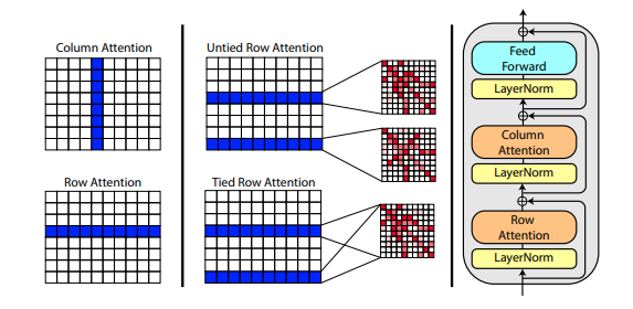
บทความใหม่โดย Roshan Rao เสนอให้ใช้ความสนใจตามแนวแกนในการฝึกอบรม MSA เมื่อพิจารณาถึงผลลัพธ์ที่ชัดเจน พื้นที่เก็บข้อมูลนี้จะใช้รูปแบบเดียวกันในส่วนท้าย โดยเฉพาะสำหรับการเอาใจใส่ตนเองของ MSA
คุณยังสามารถเชื่อมโยงความสนใจแถวของ MSA ด้วยการตั้งค่า msa_tie_row_attn = True ในการเริ่มต้นของ Alphafold2 อย่างไรก็ตาม เพื่อที่จะใช้สิ่งนี้ คุณต้องตรวจสอบให้แน่ใจว่า ถ้าคุณมี MSA จำนวนไม่เท่ากันต่อลำดับหลัก ว่าตัวพราง MSA ถูกตั้งค่าอย่างถูกต้องเป็น False สำหรับแถวที่ไม่ได้ใช้งาน
 model = Alphafold2 (
    dim = 256 ,
    depth = 2 ,
    heads = 8 ,
    dim_head = 64 ,
    msa_tie_row_attn = True # just set this to true
)การประมวลผลเทมเพลตส่วนใหญ่จะดำเนินการโดยใช้ความสนใจในแนวแกน โดยมีการให้ความสนใจแบบไขว้ตามจำนวนมิติเทมเพลต โดยส่วนใหญ่แล้วจะเป็นไปตามแผนงานเดียวกันกับแนวทางที่ดึงดูดความสนใจทุกด้านล่าสุดในการจัดหมวดหมู่วิดีโอดังที่แสดงไว้ที่นี่
 import torch
from alphafold2_pytorch import Alphafold2

model = Alphafold2 (
    dim = 256 ,
    depth = 5 ,
    heads = 8 ,
    dim_head = 64 ,
    reversible = True ,
    sparse_self_attn = False ,
    max_seq_len = 256 ,
    cross_attn_compress_ratio = 3
). cuda ()

seq = torch . randint ( 0 , 21 , ( 1 , 16 )). cuda ()
mask = torch . ones_like ( seq ). bool (). cuda ()

msa = torch . randint ( 0 , 21 , ( 1 , 10 , 16 )). cuda ()
msa_mask = torch . ones_like ( msa ). bool (). cuda ()

templates_seq = torch . randint ( 0 , 21 , ( 1 , 2 , 16 )). cuda ()
templates_coors = torch . randint ( 0 , 37 , ( 1 , 2 , 16 , 3 )). cuda ()
templates_mask = torch . ones_like ( templates_seq ). bool (). cuda ()

distogram = model (
    seq ,
    msa ,
    mask = mask ,
    msa_mask = msa_mask ,
    templates_seq = templates_seq ,
    templates_coors = templates_coors ,
    templates_mask = templates_mask
)
หากมีข้อมูลไซด์เชนอยู่ด้วย ในรูปแบบของเวกเตอร์หน่วยระหว่างพิกัด C และ C-alpha ของแต่ละเรซิดิว คุณยังสามารถส่งผ่านข้อมูลดังกล่าวได้ดังต่อไปนี้
 import torch
from alphafold2_pytorch import Alphafold2

model = Alphafold2 (
    dim = 256 ,
    depth = 5 ,
    heads = 8 ,
    dim_head = 64 ,
    reversible = True ,
    sparse_self_attn = False ,
    max_seq_len = 256 ,
    cross_attn_compress_ratio = 3
). cuda ()

seq = torch . randint ( 0 , 21 , ( 1 , 16 )). cuda ()
mask = torch . ones_like ( seq ). bool (). cuda ()

msa = torch . randint ( 0 , 21 , ( 1 , 10 , 16 )). cuda ()
msa_mask = torch . ones_like ( msa ). bool (). cuda ()

templates_seq = torch . randint ( 0 , 21 , ( 1 , 2 , 16 )). cuda ()
templates_coors = torch . randn ( 1 , 2 , 16 , 3 ). cuda ()
templates_mask = torch . ones_like ( templates_seq ). bool (). cuda ()

templates_sidechains = torch . randn ( 1 , 2 , 16 , 3 ). cuda () # unit vectors of difference of C and C-alpha coordinates

distogram = model (
    seq ,
    msa ,
    mask = mask ,
    msa_mask = msa_mask ,
    templates_seq = templates_seq ,
    templates_mask = templates_mask ,
    templates_coors = templates_coors ,
    templates_sidechains = templates_sidechains
)ฉันได้เตรียมการนำ SE3 Transformer ไปใช้ใหม่ ตามที่อธิบายโดย Fabian Fuchs ในบล็อกโพสต์เกี่ยวกับการเก็งกำไร
นอกจากนี้ บทความใหม่จาก Victor และ Welling ใช้คุณลักษณะที่ไม่แปรเปลี่ยนสำหรับการเทียบเท่า E(n) ซึ่งเข้าถึง SOTA และมีประสิทธิภาพเหนือกว่า SE3 Transformer ที่เกณฑ์มาตรฐานหลายประการ ในขณะที่เร็วกว่ามาก ฉันได้นำแนวคิดหลักจากบทความนี้มาแก้ไขให้กลายเป็นหม้อแปลงไฟฟ้า (เพิ่มความสนใจไปที่ทั้งคุณสมบัติและการอัปเดตการประสานงาน)
เครือข่ายที่เทียบเท่ากันทั้งสามเครือข่ายข้างต้นได้รับการผสานรวมแล้วและพร้อมใช้งานในพื้นที่เก็บข้อมูลสำหรับการปรับแต่งพิกัดอะตอมมิก โดยเพียงแค่ตั้งค่าไฮเปอร์พารามิเตอร์หนึ่ง structure_module_type
se3 SE3 หม้อแปลงไฟฟ้า
egnn EGNN
en E(n)-หม้อแปลงไฟฟ้า
ที่น่าสนใจสำหรับผู้อ่าน แต่ละกรอบทั้งสามยังได้รับการตรวจสอบโดยนักวิจัยเกี่ยวกับปัญหาที่เกี่ยวข้องอีกด้วย
$ python setup.py test ห้องสมุดนี้จะใช้ผลงานที่ยอดเยี่ยมของ Jonathan King ในพื้นที่เก็บข้อมูลนี้ ขอบคุณโจนาธาน!
นอกจากนี้เรายังมีข้อมูล MSA ซึ่งมีมูลค่าทั้งหมดประมาณ 3.5 TB ซึ่งดาวน์โหลดและโฮสต์โดย Archivist ซึ่งเป็นเจ้าของโครงการ The-Eye (พวกเขายังโฮสต์ข้อมูลและแบบจำลองสำหรับ Eleuther AI) โปรดพิจารณาการบริจาคหากคุณพบว่าสิ่งเหล่านี้มีประโยชน์
$ curl -s https://the-eye.eu/eleuther_staging/globus_stuffs/tree.txthttps://xukui.cn/alphafold2.html
https://moalquraishi.wordpress.com/2020/12/08/alphafold2-casp14-it-feels-like-ones-child-has-left-home/
https://www.biorxiv.org/content/10.1101/2020.12.10.419994v1.full.pdf
https://pubmed.ncbi.nlm.nih.gov/33637700/
การนำเสนอ tFold จากห้องปฏิบัติการ Tencent AI
cd downloads_folder > pip install pyrosetta_wheel_filename.whlOpenMM อำพัน
 @misc { unpublished2021alphafold2 ,
    title   = { Alphafold2 } ,
    author  = { John Jumper } ,
    year    = { 2020 } ,
    archivePrefix = { arXiv } ,
    primaryClass = { q-bio.BM }
}
@article { Rao2021.02.12.430858 ,
author = { Rao, Roshan and Liu, Jason and Verkuil, Robert and Meier, Joshua and Canny, John F. and Abbeel, Pieter and Sercu, Tom and Rives, Alexander } ,
title = { MSA Transformer } ,
year = { 2021 } ,
publisher = { Cold Spring Harbor Laboratory } ,
URL = { https://www.biorxiv.org/content/early/2021/02/13/2021.02.12.430858 } ,
journal = { bioRxiv }
} @article { Rives622803 ,
author = { Rives, Alexander and Goyal, Siddharth and Meier, Joshua and Guo, Demi and Ott, Myle and Zitnick, C. Lawrence and Ma, Jerry and Fergus, Rob } ,
title = { Biological Structure and Function Emerge from Scaling Unsupervised Learning to 250 Million Protein Sequences } ,
year = { 2019 } ,
doi = { 10.1101/622803 } ,
publisher = { Cold Spring Harbor Laboratory } ,
journal = { bioRxiv }
} @article { Elnaggar2020.07.12.199554 ,
author = { Elnaggar, Ahmed and Heinzinger, Michael and Dallago, Christian and Rehawi, Ghalia and Wang, Yu and Jones, Llion and Gibbs, Tom and Feher, Tamas and Angerer, Christoph and Steinegger, Martin and BHOWMIK, DEBSINDHU and Rost, Burkhard } ,
title = { ProtTrans: Towards Cracking the Language of Life{textquoteright}s Code Through Self-Supervised Deep Learning and High Performance Computing } ,
elocation-id = { 2020.07.12.199554 } ,
year = { 2021 } ,
doi = { 10.1101/2020.07.12.199554 } ,
publisher = { Cold Spring Harbor Laboratory } ,
URL = { https://www.biorxiv.org/content/early/2021/05/04/2020.07.12.199554 } ,
eprint = { https://www.biorxiv.org/content/early/2021/05/04/2020.07.12.199554.full.pdf } ,
journal = { bioRxiv }
} @misc { king2020sidechainnet ,
title = { SidechainNet: An All-Atom Protein Structure Dataset for Machine Learning } ,
author = { Jonathan E. King and David Ryan Koes } ,
year = { 2020 } ,
eprint = { 2010.08162 } ,
archivePrefix = { arXiv } ,
primaryClass = { q-bio.BM }
} @misc { alquraishi2019proteinnet ,
title = { ProteinNet: a standardized data set for machine learning of protein structure } ,
author = { Mohammed AlQuraishi } ,
year = { 2019 } ,
eprint = { 1902.00249 } ,
archivePrefix = { arXiv } ,
primaryClass = { q-bio.BM }
} @misc { gomez2017reversible ,
title = { The Reversible Residual Network: Backpropagation Without Storing Activations } ,
author = { Aidan N. Gomez and Mengye Ren and Raquel Urtasun and Roger B. Grosse } ,
year = { 2017 } ,
eprint = { 1707.04585 } ,
archivePrefix = { arXiv } ,
primaryClass = { cs.CV }
} @misc { fuchs2021iterative ,
title = { Iterative SE(3)-Transformers } ,
author = { Fabian B. Fuchs and Edward Wagstaff and Justas Dauparas and Ingmar Posner } ,
year = { 2021 } ,
eprint = { 2102.13419 } ,
archivePrefix = { arXiv } ,
primaryClass = { cs.LG }
} @misc { satorras2021en ,
title = { E(n) Equivariant Graph Neural Networks } ,
author = { Victor Garcia Satorras and Emiel Hoogeboom and Max Welling } ,
year = { 2021 } ,
eprint = { 2102.09844 } ,
archivePrefix = { arXiv } ,
primaryClass = { cs.LG }
} @misc { su2021roformer ,
title = { RoFormer: Enhanced Transformer with Rotary Position Embedding } ,
author = { Jianlin Su and Yu Lu and Shengfeng Pan and Bo Wen and Yunfeng Liu } ,
year = { 2021 } ,
eprint = { 2104.09864 } ,
archivePrefix = { arXiv } ,
primaryClass = { cs.CL }
} @article { Gao_2020 ,
title = { Kronecker Attention Networks } ,
ISBN = { 9781450379984 } ,
url = { http://dx.doi.org/10.1145/3394486.3403065 } ,
DOI = { 10.1145/3394486.3403065 } ,
journal = { Proceedings of the 26th ACM SIGKDD International Conference on Knowledge Discovery & Data Mining } ,
publisher = { ACM } ,
author = { Gao, Hongyang and Wang, Zhengyang and Ji, Shuiwang } ,
year = { 2020 } ,
month = { Jul }
} @article { Si2021.05.10.443415 ,
author = { Si, Yunda and Yan, Chengfei } ,
title = { Improved protein contact prediction using dimensional hybrid residual networks and singularity enhanced loss function } ,
elocation-id = { 2021.05.10.443415 } ,
year = { 2021 } ,
doi = { 10.1101/2021.05.10.443415 } ,
publisher = { Cold Spring Harbor Laboratory } ,
URL = { https://www.biorxiv.org/content/early/2021/05/11/2021.05.10.443415 } ,
eprint = { https://www.biorxiv.org/content/early/2021/05/11/2021.05.10.443415.full.pdf } ,
journal = { bioRxiv }
} @article { Costa2021.06.02.446809 ,
author = { Costa, Allan and Ponnapati, Manvitha and Jacobson, Joseph M. and Chatterjee, Pranam } ,
title = { Distillation of MSA Embeddings to Folded Protein Structures with Graph Transformers } ,
year = { 2021 } ,
doi = { 10.1101/2021.06.02.446809 } ,
publisher = { Cold Spring Harbor Laboratory } ,
URL = { https://www.biorxiv.org/content/early/2021/06/02/2021.06.02.446809 } ,
eprint = { https://www.biorxiv.org/content/early/2021/06/02/2021.06.02.446809.full.pdf } ,
journal = { bioRxiv }
} @article { Baek2021.06.14.448402 ,
author = { Baek, Minkyung and DiMaio, Frank and Anishchenko, Ivan and Dauparas, Justas and Ovchinnikov, Sergey and Lee, Gyu Rie and Wang, Jue and Cong, Qian and Kinch, Lisa N. and Schaeffer, R. Dustin and Mill{'a}n, Claudia and Park, Hahnbeom and Adams, Carson and Glassman, Caleb R. and DeGiovanni, Andy and Pereira, Jose H. and Rodrigues, Andria V. and van Dijk, Alberdina A. and Ebrecht, Ana C. and Opperman, Diederik J. and Sagmeister, Theo and Buhlheller, Christoph and Pavkov-Keller, Tea and Rathinaswamy, Manoj K and Dalwadi, Udit and Yip, Calvin K and Burke, John E and Garcia, K. Christopher and Grishin, Nick V. and Adams, Paul D. and Read, Randy J. and Baker, David } ,
title = { Accurate prediction of protein structures and interactions using a 3-track network } ,
year = { 2021 } ,
doi = { 10.1101/2021.06.14.448402 } ,
publisher = { Cold Spring Harbor Laboratory } ,
URL = { https://www.biorxiv.org/content/early/2021/06/15/2021.06.14.448402 } ,
eprint = { https://www.biorxiv.org/content/early/2021/06/15/2021.06.14.448402.full.pdf } ,
journal = { bioRxiv }
}

