pandas ta
v0.3.14b
การวิเคราะห์ทางเทคนิคของ Pandas ( Pandas TA ) เป็นห้องสมุดที่ใช้งานง่ายซึ่งใช้ประโยชน์จากแพ็คเกจแพนด้าที่มีตัวบ่งชี้มากกว่า 130 ตัวและฟังก์ชั่นยูทิลิตี้และรูปแบบเชิงเทียน Lib มากกว่า 60 TA ตัวบ่งชี้ที่ใช้กันทั่วไปจำนวนมากรวมอยู่ใน: รูปแบบเทียน ( CDL_PATTERN ), ค่าเฉลี่ยเคลื่อนที่แบบง่าย ( SMA ) การลู่เข้าคอนเวอร์เจนซ์เฉลี่ย ( MACD ), ค่าเฉลี่ยเคลื่อนที่แบบเอ็กซ์โปเนนเชียลของตัวถัง ( HMA ), Bollinger Bands ( BBands ), ปริมาณบนสมดุล ( obv ), Aroon & Aroon Oscillator ( Aroon ), บีบ ( บีบ ) และ อีกมากมาย
หมายเหตุ: ต้องติดตั้ง TA lib เพื่อใช้รูปแบบเชิงเทียน ทั้งหมด pip install TA-Lib หากไม่ได้ติดตั้ง TA lib จะมีเพียงรูปแบบเชิงเทียนในตัวเท่านั้น
talib=Falseta.stdev(df["close"], length=30, talib=False)import_dir ภายใต้ /pandas_ta/custom.pyta.tsignals ของ Pandas TAlookahead=False เพื่อปิดการใช้งานPandas TA ตรวจสอบว่าผู้ใช้มีแพ็คเกจการซื้อขายทั่วไปที่ติดตั้งหรือไม่รวมถึง แต่ไม่ จำกัด เพียง: TA lib , Vector BT , Yfinance ... ซึ่งส่วนใหญ่ เป็นการทดลอง และมีแนวโน้มที่จะแตกหักจนกว่าจะมีความเสถียรมากขึ้น
help(ta.ticker) และ help(ta.yf) และตัวอย่างด้านล่าง เวอร์ชัน pip คือการเปิดตัวที่เสถียรครั้งสุดท้าย เวอร์ชัน: 0.3.14B
$ pip install pandas_taทางเลือกที่ดีที่สุด! เวอร์ชัน: 0.3.14B
$ pip install -U git+https://github.com/twopirllc/pandas-taนี่คือ เวอร์ชันการพัฒนา ที่อาจมีข้อบกพร่องและผลข้างเคียงอื่น ๆ ที่ไม่พึงประสงค์ ใช้ความเสี่ยงของตัวเอง!
$ pip install -U git+https://github.com/twopirllc/pandas-ta.git@development import pandas as pd
import pandas_ta as ta
df = pd . DataFrame () # Empty DataFrame
# Load data
df = pd . read_csv ( "path/to/symbol.csv" , sep = "," )
# OR if you have yfinance installed
df = df . ta . ticker ( "aapl" )
# VWAP requires the DataFrame index to be a DatetimeIndex.
# Replace "datetime" with the appropriate column from your DataFrame
df . set_index ( pd . DatetimeIndex ( df [ "datetime" ]), inplace = True )
# Calculate Returns and append to the df DataFrame
df . ta . log_return ( cumulative = True , append = True )
df . ta . percent_return ( cumulative = True , append = True )
# New Columns with results
df . columns
# Take a peek
df . tail ()
# vv Continue Post Processing vv อาร์กิวเมนต์ตัวบ่งชี้ บางอย่าง ได้รับการจัดลำดับใหม่เพื่อความสอดคล้อง ใช้ help(ta.indicator_name) สำหรับข้อมูลเพิ่มเติมหรือทำการร้องขอการดึงเพื่อปรับปรุงเอกสาร
 import pandas as pd
import pandas_ta as ta

# Create a DataFrame so 'ta' can be used.
df = pd . DataFrame ()

# Help about this, 'ta', extension
help ( df . ta )

# List of all indicators
df . ta . indicators ()

# Help about an indicator such as bbands
help ( ta . bbands ) ขอบคุณที่ใช้ Pandas TA !
$ pip install -U git+https://github.com/twopirllc/pandas-taขอบคุณสำหรับผลงานของคุณ!
Pandas TA มี "สไตล์" หลักสามรูปแบบของตัวบ่งชี้ทางเทคนิคการประมวลผลสำหรับกรณีการใช้งานและ/หรือข้อกำหนดของคุณ พวกเขาคือ: มาตรฐาน ส่วนขยาย DataFrame และ กลยุทธ์ Pandas TA แต่ละคนมีระดับที่เพิ่มขึ้นของสิ่งที่เป็นนามธรรมเพื่อความสะดวกในการใช้งาน เมื่อคุณคุ้นเคยกับ Pandas TA มากขึ้นความเรียบง่ายและความเร็วในการใช้ กลยุทธ์ Pandas TA อาจชัดเจนขึ้น นอกจากนี้คุณสามารถสร้างตัวบ่งชี้ของคุณเองผ่านการผูกมัดหรือองค์ประกอบ สุดท้ายตัวบ่งชี้แต่ละตัวจะส่งคืน ซีรีส์ หรือ DataFrame ในรูปแบบขีดล่างตัวพิมพ์ใหญ่โดยไม่คำนึงถึงสไตล์
คุณกำหนดคอลัมน์อินพุตอย่างชัดเจนและดูแลเอาต์พุต
sma10 = ta.sma(df["Close"], length=10)SMA_10donchiandf = ta.donchian(df["HIGH"], df["low"], lower_length=10, upper_length=15)DC_10_15 และชื่อคอลัมน์: DCL_10_15, DCM_10_15, DCU_10_15ema10_ohlc4 = ta.ema(ta.ohlc4(df["Open"], df["High"], df["Low"], df["Close"]), length=10)EMA_10 หากจำเป็นคุณอาจต้องตั้งชื่อโดยไม่ซ้ำกัน การโทร df.ta จะช่วยลดระดับ OHLCVA ไปยัง OHLCVA โดยอัตโนมัติ: เปิด, สูง, ต่ำ, ปิด, ปริมาตร , adj_close โดยค่าเริ่มต้น df.ta จะใช้ OHLCVA สำหรับอาร์กิวเมนต์ตัวบ่งชี้ที่ไม่จำเป็นต้องระบุคอลัมน์อินพุตโดยตรง
sma10 = df.ta.sma(length=10)SMA_10ema10_ohlc4 = df.ta.ema(close=df.ta.ohlc4(), length=10, suffix="OHLC4")EMA_10_OHLC4close=df.ta.ohlc4()donchiandf = df.ta.donchian(lower_length=10, upper_length=15)DC_10_15 และชื่อคอลัมน์: DCL_10_15, DCM_10_15, DCU_10_15 เช่นเดียวกับสามตัวอย่างสุดท้าย แต่ต่อท้ายผลลัพธ์โดยตรงกับ DataFrame df
df.ta.sma(length=10, append=True)df : SMA_10df.ta.ema(close=df.ta.ohlc4(append=True), length=10, suffix="OHLC4", append=True)close=df.ta.ohlc4()df.ta.donchian(lower_length=10, upper_length=15, append=True)df ด้วยชื่อคอลัมน์: DCL_10_15, DCM_10_15, DCU_10_15 กลยุทธ์ Pandas TA เป็นกลุ่มตัวชี้วัดที่มีชื่อที่จะดำเนินการโดยวิธี กลยุทธ์ กลยุทธ์ทั้งหมดใช้ mulitprocessing ยกเว้น เมื่อใช้พารามิเตอร์ col_names (ดูด้านล่าง) มี กลยุทธ์ ประเภทต่าง ๆ ที่ระบุไว้ในส่วนต่อไปนี้
 # (1) Create the Strategy
MyStrategy = ta . Strategy (
    name = "DCSMA10" ,
    ta = [
        { "kind" : "ohlc4" },
        { "kind" : "sma" , "length" : 10 },
        { "kind" : "donchian" , "lower_length" : 10 , "upper_length" : 15 },
        { "kind" : "ema" , "close" : "OHLC4" , "length" : 10 , "suffix" : "OHLC4" },
    ]
)

# (2) Run the Strategy
df . ta . strategy ( MyStrategy , ** kwargs )คลาส กลยุทธ์ เป็นวิธีง่ายๆในการตั้งชื่อและจัดกลุ่มตัวบ่งชี้ TA ที่คุณชื่นชอบโดยใช้ คลาสข้อมูล Pandas TA มาพร้อมกับสองกลยุทธ์พื้นฐานที่สร้างไว้ล่วงหน้าเพื่อช่วยให้คุณเริ่มต้นได้: Allstrategy และ Commonstrategy กลยุทธ์ สามารถทำได้ง่ายเหมือน commonstrategy หรือซับซ้อนเท่าที่จำเป็นโดยใช้องค์ประกอบ/การผูกมัด
df โดยอัตโนมัติดูตัวอย่างกลยุทธ์ Pandas TA สำหรับตัวอย่างรวมถึง องค์ประกอบตัวบ่งชี้/การผูกมัด
{"kind": "indicator name"} อย่าลืม ตรวจสอบการสะกดคำของคุณ # Running the Builtin CommonStrategy as mentioned above
df . ta . strategy ( ta . CommonStrategy )
# The Default Strategy is the ta.AllStrategy. The following are equivalent:
df . ta . strategy ()
df . ta . strategy ( "All" )
df . ta . strategy ( ta . AllStrategy ) # List of indicator categories
df . ta . categories
# Running a Categorical Strategy only requires the Category name
df . ta . strategy ( "Momentum" ) # Default values for all Momentum indicators
df . ta . strategy ( "overlap" , length = 42 ) # Override all Overlap 'length' attributes # Create your own Custom Strategy
CustomStrategy = ta . Strategy (
name = "Momo and Volatility" ,
description = "SMA 50,200, BBANDS, RSI, MACD and Volume SMA 20" ,
ta = [
{ "kind" : "sma" , "length" : 50 },
{ "kind" : "sma" , "length" : 200 },
{ "kind" : "bbands" , "length" : 20 },
{ "kind" : "rsi" },
{ "kind" : "macd" , "fast" : 8 , "slow" : 21 },
{ "kind" : "sma" , "close" : "volume" , "length" : 20 , "prefix" : "VOLUME" },
]
)
# To run your "Custom Strategy"
df . ta . strategy ( CustomStrategy ) วิธี กลยุทธ์ Pandas TA ใช้ การประมวลผลแบบหลายโปรเซสเซอร์ สำหรับการประมวลผลตัวบ่งชี้จำนวนมากของกลยุทธ์ทุกประเภทด้วย ข้อยกเว้นหนึ่งข้อ! เมื่อใช้พารามิเตอร์ col_names เพื่อเปลี่ยนชื่อคอลัมน์ผลลัพธ์ตัวบ่งชี้ในอาร์เรย์ ta จะถูกเรียกใช้ตามลำดับ
 # VWAP requires the DataFrame index to be a DatetimeIndex.
# * Replace "datetime" with the appropriate column from your DataFrame
df . set_index ( pd . DatetimeIndex ( df [ "datetime" ]), inplace = True )

# Runs and appends all indicators to the current DataFrame by default
# The resultant DataFrame will be large.
df . ta . strategy ()
# Or the string "all"
df . ta . strategy ( "all" )
# Or the ta.AllStrategy
df . ta . strategy ( ta . AllStrategy )

# Use verbose if you want to make sure it is running.
df . ta . strategy ( verbose = True )

# Use timed if you want to see how long it takes to run.
df . ta . strategy ( timed = True )

# Choose the number of cores to use. Default is all available cores.
# For no multiprocessing, set this value to 0.
df . ta . cores = 4

# Maybe you do not want certain indicators.
# Just exclude (a list of) them.
df . ta . strategy ( exclude = [ "bop" , "mom" , "percent_return" , "wcp" , "pvi" ], verbose = True )

# Perhaps you want to use different values for indicators.
# This will run ALL indicators that have fast or slow as parameters.
# Check your results and exclude as necessary.
df . ta . strategy ( fast = 10 , slow = 50 , verbose = True )

# Sanity check. Make sure all the columns are there
df . columns โปรดจำไว้ว่า สิ่งเหล่านี้จะไม่ใช้ การประมวลผลหลายครั้ง
 NonMPStrategy = ta . Strategy (
    name = "EMAs, BBs, and MACD" ,
    description = "Non Multiprocessing Strategy by rename Columns" ,
    ta = [
        { "kind" : "ema" , "length" : 8 },
        { "kind" : "ema" , "length" : 21 },
        { "kind" : "bbands" , "length" : 20 , "col_names" : ( "BBL" , "BBM" , "BBU" )},
        { "kind" : "macd" , "fast" : 8 , "slow" : 21 , "col_names" : ( "MACD" , "MACD_H" , "MACD_S" )}
    ]
)
# Run it
df . ta . strategy ( NonMPStrategy ) # Set ta to default to an adjusted column, 'adj_close', overriding default 'close'.
df . ta . adjusted = "adj_close"
df . ta . sma ( length = 10 , append = True )
# To reset back to 'close', set adjusted back to None.
df . ta . adjusted = None # List of Pandas TA categories.
df . ta . categories # Set the number of cores to use for strategy multiprocessing
# Defaults to the number of cpus you have.
df . ta . cores = 4
# Set the number of cores to 0 for no multiprocessing.
df . ta . cores = 0
# Returns the number of cores you set or your default number of cpus.
df . ta . cores # The 'datetime_ordered' property returns True if the DataFrame
# index is of Pandas datetime64 and df.index[0] < df.index[-1].
# Otherwise it returns False.
df . ta . datetime_ordered # Sets the Exchange to use when calculating the last_run property. Default: "NYSE"
df . ta . exchange
# Set the Exchange to use.
# Available Exchanges: "ASX", "BMF", "DIFX", "FWB", "HKE", "JSE", "LSE", "NSE", "NYSE", "NZSX", "RTS", "SGX", "SSE", "TSE", "TSX"
df . ta . exchange = "LSE" # Returns the time Pandas TA was last run as a string.
df . ta . last_run # The 'reverse' is a helper property that returns the DataFrame
# in reverse order.
df . ta . reverse # Applying a prefix to the name of an indicator.
prehl2 = df . ta . hl2 ( prefix = "pre" )
print ( prehl2 . name ) # "pre_HL2"
# Applying a suffix to the name of an indicator.
endhl2 = df . ta . hl2 ( suffix = "post" )
print ( endhl2 . name ) # "HL2_post"
# Applying a prefix and suffix to the name of an indicator.
bothhl2 = df . ta . hl2 ( prefix = "pre" , suffix = "post" )
print ( bothhl2 . name ) # "pre_HL2_post" # Returns the time range of the DataFrame as a float.
# By default, it returns the time in "years"
df . ta . time_range
# Available time_ranges include: "years", "months", "weeks", "days", "hours", "minutes". "seconds"
df . ta . time_range = "days"
df . ta . time_range # prints DataFrame time in "days" as float # Sets the DataFrame index to UTC format.
df . ta . to_utc import numpy as np
# Add constant '1' to the DataFrame
df . ta . constants ( True , [ 1 ])
# Remove constant '1' to the DataFrame
df . ta . constants ( False , [ 1 ])
# Adding constants for charting
import numpy as np
chart_lines = np . append ( np . arange ( - 4 , 5 , 1 ), np . arange ( - 100 , 110 , 10 ))
df . ta . constants ( True , chart_lines )
# Removing some constants from the DataFrame
df . ta . constants ( False , np . array ([ - 60 , - 40 , 40 , 60 ])) # Prints the indicators and utility functions
df . ta . indicators ()
# Returns a list of indicators and utility functions
ind_list = df . ta . indicators ( as_list = True )
# Prints the indicators and utility functions that are not in the excluded list
df . ta . indicators ( exclude = [ "cg" , "pgo" , "ui" ])
# Returns a list of the indicators and utility functions that are not in the excluded list
smaller_list = df . ta . indicators ( exclude = [ "cg" , "pgo" , "ui" ], as_list = True ) # Download Chart history using yfinance. (pip install yfinance) https://github.com/ranaroussi/yfinance
# It uses the same keyword arguments as yfinance (excluding start and end)
df = df . ta . ticker ( "aapl" ) # Default ticker is "SPY"
# Period is used instead of start/end
# Valid periods: 1d,5d,1mo,3mo,6mo,1y,2y,5y,10y,ytd,max
# Default: "max"
df = df . ta . ticker ( "aapl" , period = "1y" ) # Gets this past year
# History by Interval by interval (including intraday if period < 60 days)
# Valid intervals: 1m,2m,5m,15m,30m,60m,90m,1h,1d,5d,1wk,1mo,3mo
# Default: "1d"
df = df . ta . ticker ( "aapl" , period = "1y" , interval = "1wk" ) # Gets this past year in weeks
df = df . ta . ticker ( "aapl" , period = "1mo" , interval = "1h" ) # Gets this past month in hours
# BUT WAIT!! THERE'S MORE!!
help ( ta . yf ) รูปแบบที่ ไม่เป็นตัวหนา ต้องการการติดตั้ง ta-lib: pip install TA-Lib
 # Get all candle patterns (This is the default behaviour)
df = df . ta . cdl_pattern ( name = "all" )

# Get only one pattern
df = df . ta . cdl_pattern ( name = "doji" )

# Get some patterns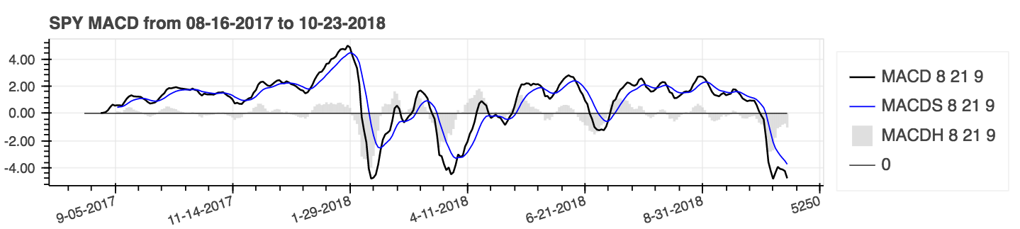
df = df . ta . cdl_pattern ( name = [ "doji" , "inside" ])ta.linreg(series, r=True)lazybear=Truedf.ta.strategy()| ความแตกต่างการบรรจบกันเฉลี่ย (MACD) |
|---|
 |
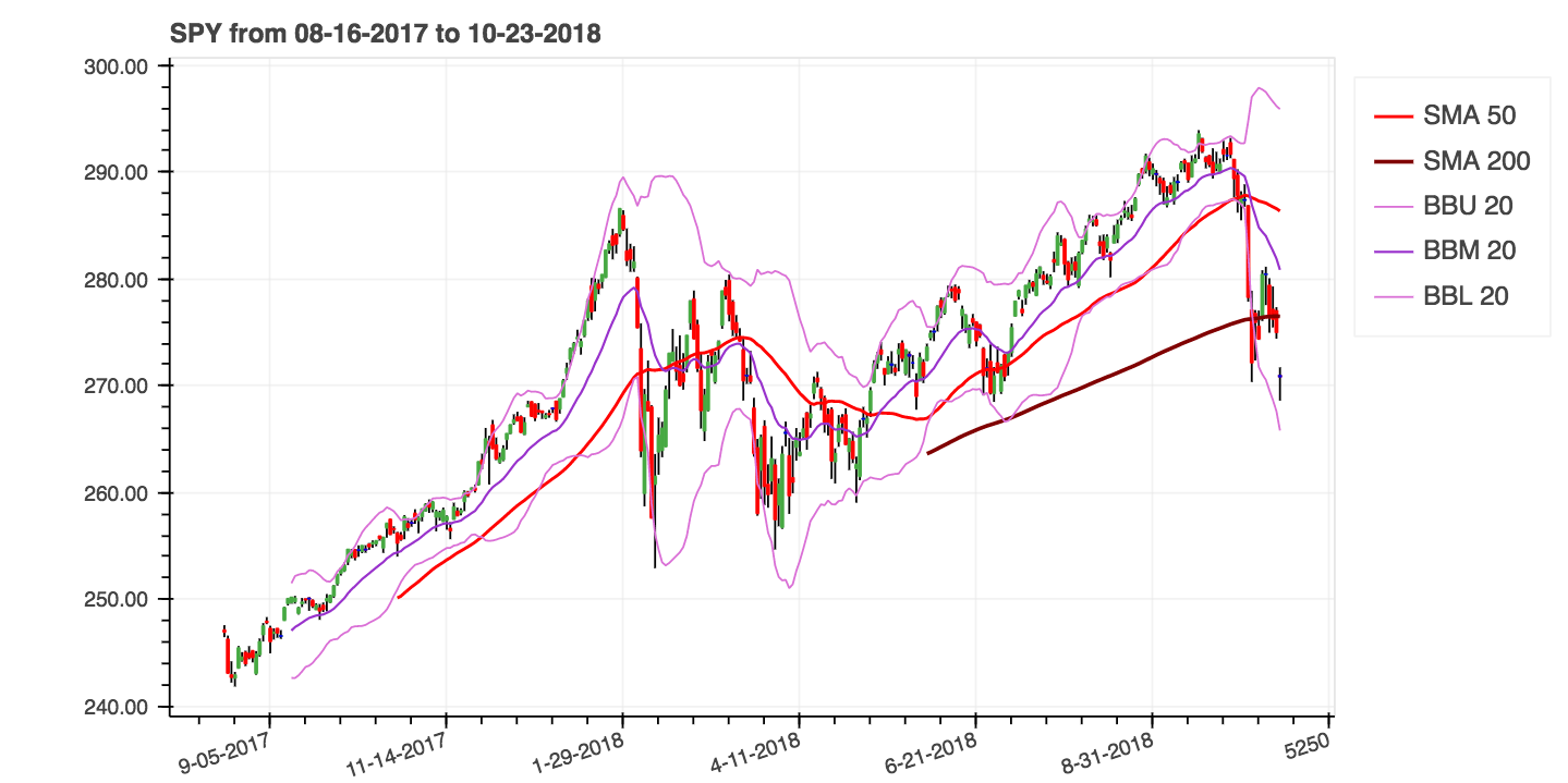
help(ta.ichimoku)lookahead=False ลดลงคอลัมน์ Chikou Span เพื่อป้องกันการรั่วไหลของข้อมูลที่อาจเกิดขึ้น| ค่าเฉลี่ยเคลื่อนที่อย่างง่าย (SMA) และ Bollinger Bands (BBands) |
|---|
|
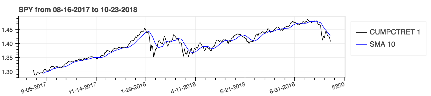
ใช้พารามิเตอร์: สะสม = จริง สำหรับผลลัพธ์สะสม
| เปอร์เซ็นต์ผลตอบแทน (สะสม) ที่มี ค่าเฉลี่ยเคลื่อนที่อย่างง่าย (SMA) |
|---|
 |
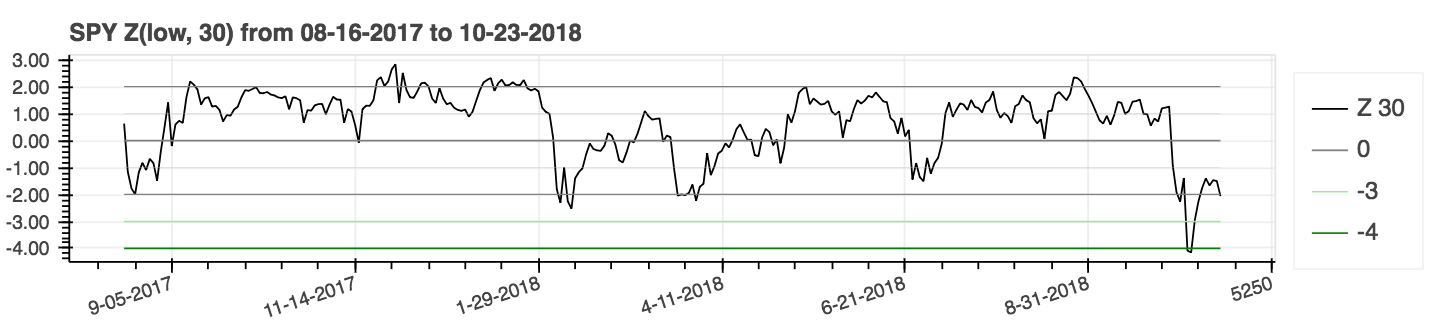
| คะแนน z |
|---|
 |
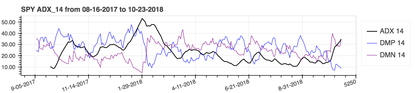
lookahead=False เพื่อปิดการใช้งานศูนย์และลบการรั่วไหลของข้อมูลที่อาจเกิดขึ้น| ดัชนีการเคลื่อนไหวทิศทางเฉลี่ย (ADX) |
|---|
 |
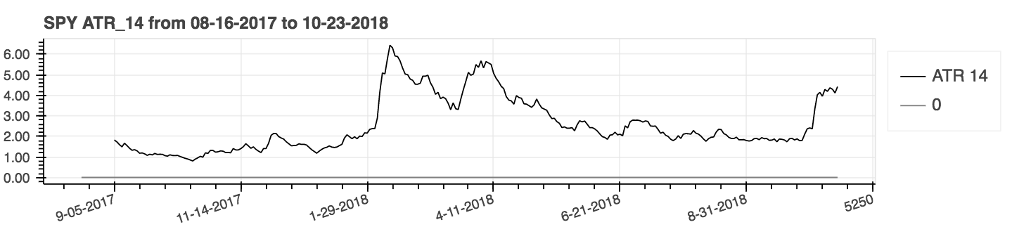
| ช่วงจริงเฉลี่ย (ATR) |
|---|
 |
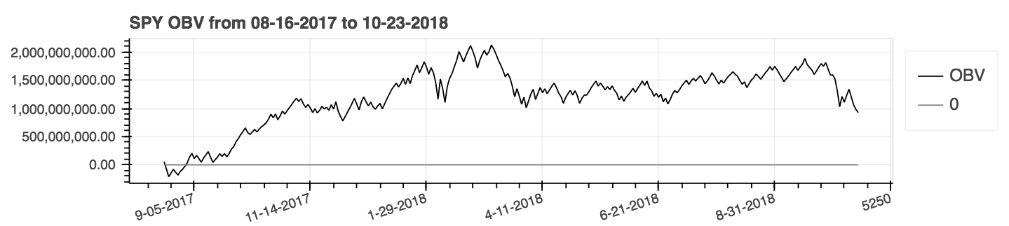
| ระดับความสมดุล (obv) |
|---|
 |
ตัวชี้วัดประสิทธิภาพ เป็นส่วนเสริม ใหม่ ของแพ็คเกจและอาจไม่น่าเชื่อถือ ใช้ความเสี่ยงของคุณเอง ตัวชี้วัดเหล่านี้กลับมา ลอย และ ไม่ได้ เป็นส่วนหนึ่งของส่วนขยาย DataFrame พวกเขาเรียกว่าวิธีมาตรฐาน ตัวอย่างเช่น:
 import pandas_ta as ta
result = ta . cagr ( df . close ) เพื่อการรวม ที่ง่ายขึ้น ด้วยวิธีการของ VectorBT from_signals วิธี ta.trend_return ได้ถูกแทนที่ด้วยวิธี ta.tsignals เพื่อลดความซับซ้อนของการสร้างสัญญาณการซื้อขาย สำหรับตัวอย่างที่ครอบคลุมให้ดูตัวอย่าง Jupyter Notebook Backtest backtest กับ Pandas TA ในไดเรกทอรีตัวอย่าง
 import pandas as pd
import pandas_ta as ta
import vectorbt as vbt

df = pd . DataFrame (). ta . ticker ( "AAPL" ) # requires 'yfinance' installed

# Create the "Golden Cross"
df [ "GC" ] = df . ta . sma ( 50 , append = True ) > df . ta . sma ( 200 , append = True )

# Create boolean Signals(TS_Entries, TS_Exits) for vectorbt
golden = df . ta . tsignals ( df . GC , asbool = True , append = True )

# Sanity Check (Ensure data exists)
print ( df )

# Create the Signals Portfolio
pf = vbt . Portfolio . from_signals ( df . close , entries = golden . TS_Entries , exits = golden . TS_Exits , freq = "D" , init_cash = 100_000 , fees = 0.0025 , slippage = 0.0025 )

# Print Portfolio Stats and Return Stats
print ( pf . stats ())
print ( pf . returns_stats ())mamode Kwarg ด้วยตัวเลือก เฉลี่ยเคลื่อนที่ มากขึ้นด้วยฟังก์ชั่น ยูทิลิตี้เฉลี่ยเคลื่อนที่ ta.ma() เพื่อความเรียบง่าย ตัวเลือก ทั้งหมดเป็น ค่าเฉลี่ยเคลื่อนที่ เดียว นี่คือยูทิลิตี้ภายในที่ใช้โดยตัวบ่งชี้ที่มี mamode kwarg ซึ่งรวมถึงตัวชี้วัด: Accbands , AMAT , AOBV , ATR , BBANDS , BIAS , EFI , HILO , KC , NATR , QQE , RVI และ Thermo ; พารามิเตอร์ mamode เริ่มต้นไม่เปลี่ยนแปลง อย่างไรก็ตามผู้ใช้สามารถใช้ ta.ma() ได้เช่นกันหากจำเป็น สำหรับข้อมูลเพิ่มเติม: help(ta.ma)to_utc เพื่อแปลงดัชนี DataFrame เป็น UTC ดู: help(ta.to_utc) ตอนนี้ เป็นคุณสมบัติ pandas ta dataframe เพื่อแปลงดัชนี dataframe เป็น UTC ได้อย่างง่ายดาย close > sma(close, 50) มันจะส่งคืนแนวโน้มรายการการค้าและการออกจากเทรนด์การค้าเพื่อให้เข้ากันได้กับ vectorbt โดยการตั้งค่า asbool=True เพื่อรับรายการการค้าบูลีนและออก ดู help(ta.tsignals) help(ta.alma) บัญชีการซื้อขายหรือกองทุน ดู help(ta.drawdown)help(ta.cdl_pattern)help(ta.cdl_z)help(ta.cti)help(ta.xsignals)help(ta.dm)help(ta.ebsw)help(ta.jma)help(ta.kvo)help(ta.stc)help(ta.squeeze_pro)df.ta.strategy() ด้วยเหตุผลด้านประสิทธิภาพ ดู help(ta.td_seq)help(ta.tos_stdevall)help(ta.vhf) mamode เปลี่ยนชื่อเป็น mode ดู help(ta.accbands)mamode ด้วยค่าเริ่มต้น " RMA " และด้วยตัวเลือก mamode เดียวกันกับการซื้อขาย View อาร์กิวเมนต์ใหม่ lensig ดังนั้นมันจึงทำงานเหมือนตัวบ่งชี้ ADX ในตัวของ TradingView ดู help(ta.adx)drift ท์และชื่อคอลัมน์เชิงพรรณนามากขึ้นmamode เริ่มต้นคือตอนนี้ " RMA " และด้วยตัวเลือก mamode เดียวกับการซื้อขาย ดู help(ta.atr)ddoff เพื่อควบคุมองศาอิสระ รวมถึง BB เปอร์เซ็นต์ (BBP) เป็นคอลัมน์สุดท้าย ค่าเริ่มต้นคือ 0. ดู help(ta.bbands)ln เพื่อใช้ลอการิทึมธรรมชาติ (จริง) แทนลอการิทึมมาตรฐาน (เท็จ) ค่าเริ่มต้นเป็นเท็จ ดู help(ta.chop)tvmode ด้วยค่าเริ่มต้น True เมื่อ tvmode=False CKSP จะใช้“ ผู้ค้าทางเทคนิคใหม่” ที่มีค่าเริ่มต้น ดู help(ta.cksp)talib จะใช้เวอร์ชันของ Ta Lib และหากติดตั้ง TA lib ค่าเริ่มต้นเป็นจริง ดู help(ta.cmo)strict หากซีรีส์ลดลงอย่างต่อเนื่องตลอดระยะเวลา length ด้วยการคำนวณที่เร็วขึ้น ค่าเริ่มต้น: False อาร์กิวเมนต์ percent ได้ถูกเพิ่มด้วยค่าเริ่มต้นไม่มี ดู help(ta.decreasing)strict หากซีรีส์เพิ่มขึ้นอย่างต่อเนื่องตลอดระยะเวลา length ด้วยการคำนวณที่เร็วขึ้น ค่าเริ่มต้น: False อาร์กิวเมนต์ percent ได้ถูกเพิ่มด้วยค่าเริ่มต้นไม่มี ดู help(ta.increasing)help(ta.kvo)as_strided หรือวิธีการเลื่อนใหม่ sliding_window_view ที่ใหม่กว่า สิ่งนี้ควรแก้ไขปัญหาเกี่ยวกับ Google Colab และมีการอัปเดตการพึ่งพาการพึ่งพาล่าช้าเช่นเดียวกับการพึ่งพาของ TensorFlow ตามที่กล่าวไว้ในประเด็น #285 และ #329asmode เปิดใช้งานเป็นเวอร์ชันของ MACD ค่าเริ่มต้นเป็นเท็จ ดู help(ta.macd)sar ของ TradingView อาร์กิวเมนต์ใหม่ af0 เพื่อเริ่มต้นปัจจัยการเร่งความเร็ว ดู help(ta.psar)mamode เป็นตัวเลือก ค่าเริ่มต้นคือ SMA เพื่อให้ตรงกับ TA Lib ดู help(ta.ppo)signal ด้วยค่าเริ่มต้น 13 และโหมด MAMODE mamode ที่มี EMA เริ่มต้นเป็นอาร์กิวเมนต์ ดู help(ta.tsi)help(ta.vp)help(ta.vwma)anchor ค่าเริ่มต้น: "D" สำหรับ "รายวัน" ดูนามแฝงออฟเซ็ต Timeseries สำหรับตัวเลือกเพิ่มเติม ต้องการให้ ดัชนี DataFrame เป็น DateTimeIndex ดู help(ta.vwap)help(ta.vwma)Z_length เป็น ZS_length ดู help(ta.zscore)TA-LIB ดั้งเดิม | TradingView | แผนภูมิเซียร่า MQL5 | FM Labs | Pro Pro Real Code | ผู้ใช้ 42
รู้สึกใจกว้างเหมือนแพ็คเกจหรือต้องการเห็นมันกลายเป็นแพ็คเกจที่เป็นผู้ใหญ่มากขึ้น?


