dsc 2 22 03 MLE gaussian lab bain trial jan19

正态分布的 MLE - 实验室

介绍

在本实验中，我们将实践我们在上一课中看到的数学公式，以了解 MLE 如何处理正态分布。

目标

您将能够：

• 理解并描述 MLE 如何与正态分布一起工作
• 将正态分布拟合到给定数据，识别均值和方差
• 直观地比较拟合分布与真实分布

注意： *所有 MLE 方程的详细推导和证明可以在这个网站上看到。 *

Python 中的最大似然估计

下面让我们看一个使用 Python 进行 MLE 和分布拟合的示例。这里scipy.stats.norm.fit使用最大似然估计计算分布参数。

导入必要的库

 from scipy . stats import norm # for generating sample data and fitting distributions
import matplotlib . pyplot as plt
plt . style . use ( 'seaborn' )
import numpy as np

从均值 0 和标准差 1 的正态分布生成 200 个随机样本的数组

 sample = None

通过 MLE 进行分布拟合

- 使用stats.norm.fit(data)来拟合上述数据的分布。

- 这将通过 MLE 方法返回两个参数的列表：(mean,:parameters[0] and std:parameters[1])

 param = None

#param[0], param[1]
# (0.08241224761452863, 1.002987490235812)

根据 a) 实际数据参数 b) 拟合参数计算 PDF，其中x = np.linspace(-5,5,100)

 x = np . linspace ( - 5 , 5 , 100 )

# Generate the pdf from fitted parameters (fitted distribution)
fitted_pdf = None
# Generate the pdf without fitting (normal distribution non fitted)
normal_pdf = None

可视化两个 PDF

 # Your code here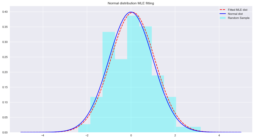 

 #  Your comments/observations 

概括

在这个简短的实验中，我们研究了高斯环境中的贝叶斯设置，即当基础随机变量呈正态分布时。我们了解到，MLE 可以通过最大化预期均值的可能性来估计正态分布的未知参数。预期平均值非常接近该参数空间内非拟合正态分布的平均值。我们将在这种理解的基础上继续学习如何使用朴素贝叶斯分类器来估计数据分布中存在的许多类别的方法。