該存儲庫的目的是跟踪我學到的一些整潔的GGPLOT2技巧。這假設您已經熟悉GGPLOT2的基礎知識,並且可以構建自己的一些不錯的圖。如果沒有,請在您的leasure中仔細閱讀這本書。
我並不是很光榮地排版地塊和專業的主題和調色板,所以您必須原諒我。 mpg數據集的繪圖非常通用,因此您會在閱讀時看到很多。擴展程序包很棒,我已經涉足自己,但是我會嘗試將自己限制在這裡的Vanilla GGPLOT2技巧。
目前,這主要是只讀的技巧,但我稍後可能會決定將它們放入其他文件中的單獨組中。
通過加載庫並設置繪圖主題。這裡的第一個技巧是使用theme_set()為整個文檔中的所有圖設置主題。如果您發現自己為每個情節設置一個非常冗長的主題,那麼這裡是設置所有常見設置的地方。然後再也不會寫一本主題元素的小說1 !
library( ggplot2 )
library( scales )

theme_set(
  # Pick a starting theme
  theme_gray() +
  # Add your favourite elements
  theme(
    axis.line        = element_line(),
    panel.background = element_rect( fill = " white " ),
    panel.grid.major = element_line( " grey95 " , linewidth = 0.25 ),
    legend.key       = element_rect( fill = NA )
  )
)?aes文檔沒有告訴您,但是您可以將mapping參數拼寫為ggplot2。這意味著什麼?好吧,這意味著您可以在旅途中撰寫mapping論點!!! 。如果您需要偶爾需要回收美學,這一點尤其令人討厭。
 my_mapping <- aes( x = foo , y = bar )

aes( colour = qux , !!! my_mapping )
# > Aesthetic mapping:
# > * `x`      -> `foo`
# > * `y`      -> `bar`
# > * `colour` -> `qux`我個人最喜歡的用途是使fill顏色與colour相匹配,但略帶2 。在這種情況下,我們將使用延遲的評估系統, after_scale() ,在此之後的部分中您會看到更多。在本文檔中,我將重複幾次此技巧。
 my_fill <- aes( fill = after_scale(alpha( colour , 0.3 )))

ggplot( mpg , aes( displ , hwy )) +
  geom_point(aes( colour = factor ( cyl ), !!! my_fill ), shape = 21 )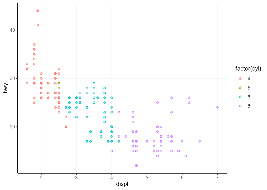
您可能會發現自己在某種情況下被要求進行少量變量的熱圖。通常,順序尺度從光到黑暗,反之亦然,這使得文字很難閱讀。我們可以設計一種方法,可以在黑暗的背景上自動以白色寫文本,而在光背景上為黑色。下面的功能考慮了顏色的輕度值,並根據該輕度返回黑色或白色。
 contrast <- function ( colour ) {
  out   <- rep( " black " , length( colour ))
  light <- farver :: get_channel( colour , " l " , space = " hcl " )
  out [ light < 50 ] <- " white "
  out
}現在,我們可以使美學按需要插入圖層的mapping參數中。
autocontrast <- aes( colour = after_scale(contrast( fill )))最後,我們可以測試自動對比度。您可能會注意到它適應了比例,因此您無需為此做很多條件格式。
cors <- cor( mtcars )
# Melt matrix
df <- data.frame (
col = colnames( cors )[as.vector(col( cors ))],
row = rownames( cors )[as.vector(row( cors ))],
value = as.vector( cors )
)
# Basic plot
p <- ggplot( df , aes( row , col , fill = value )) +
geom_raster() +
geom_text(aes( label = round( value , 2 ), !!! autocontrast )) +
coord_equal()
p + scale_fill_viridis_c( direction = 1 )
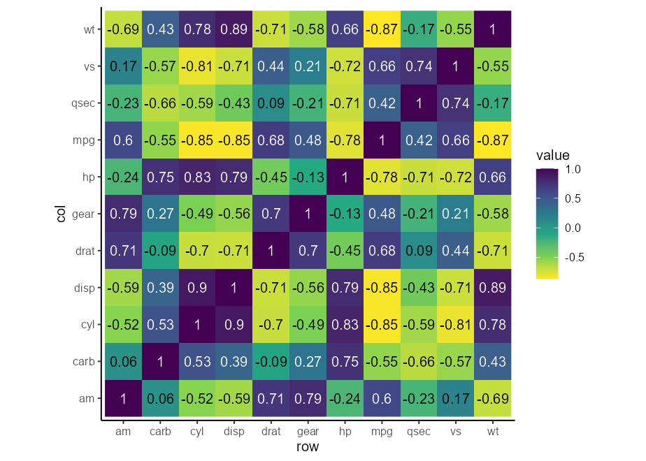
p + scale_fill_viridis_c( direction = - 1 )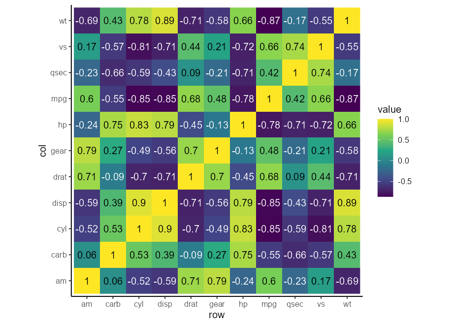
有一些擴展名提供了一半的事物版本。在我所知道的那些人中,Ghalves和See Package提供了一些半geoms。
這是濫用延遲評估系統以製造自己的方法。如果您不願意僅僅對此功能承擔額外的依賴,那麼這可能會派上用場。
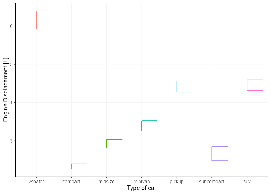
簡單的盒子是框圖。您可以將xmin或xmax設置為after_scale(x)以分別保留Boxplot的左右部分。這仍然可以與position = "dodge"效果很好。
 # A basic plot to reuse for examples
p <- ggplot( mpg , aes( class , displ , colour = class , !!! my_fill )) +
  guides( colour = " none " , fill = " none " ) +
  labs( y = " Engine Displacement [L] " , x = " Type of car " )

p + geom_boxplot(aes( xmin = after_scale( x )))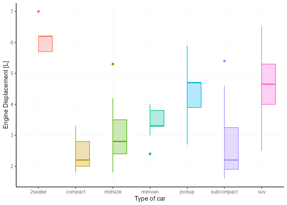
適用於盒子圖的同一件事也適用於錯誤欄。
 p + geom_errorbar(
  stat = " summary " ,
  fun.data = mean_se ,
  aes( xmin = after_scale( x ))
)
我們可以再次為小提琴圖做同樣的事情,但是該層抱怨不知道xmin美學。它確實使用了這種美學,但只有在設置了數據之後,因此它不打算是用戶可訪問的美學。我們可以通過將xmin默認值更新為NULL來使警告保持沉默,這意味著它不會抱怨,但如果不存在,也不會使用它。
update_geom_defaults( " violin " , list ( xmin = NULL ))

p + geom_violin(aes( xmin = after_scale( x )))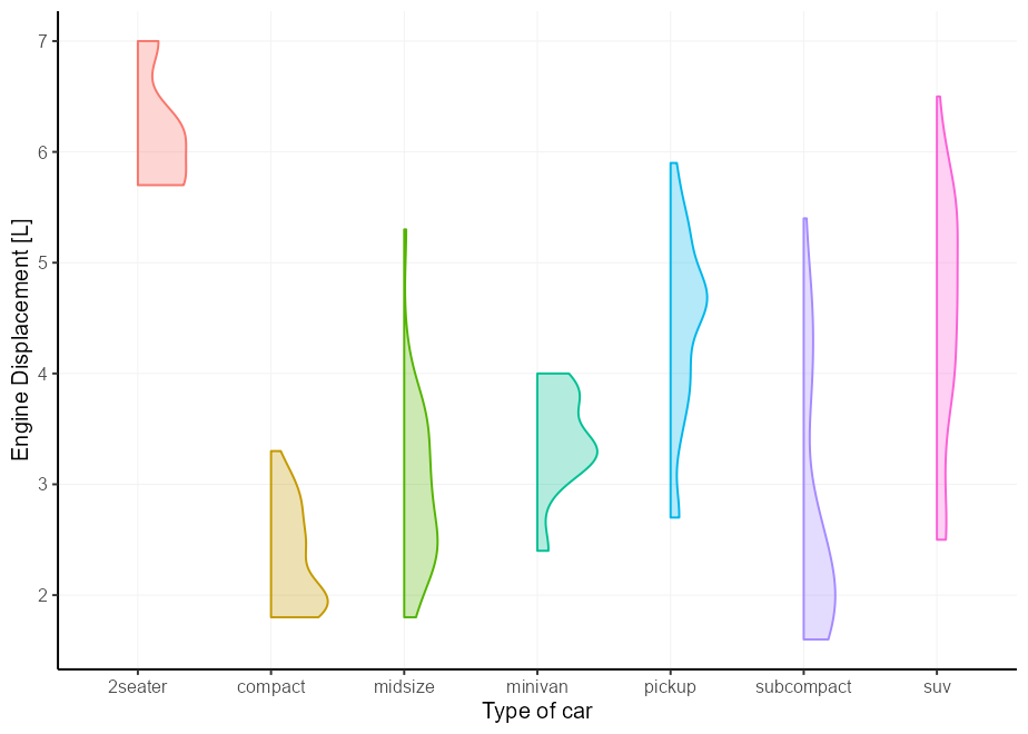
這次不是作為讀者的練習,但是我只是想展示如果您將兩半結合併希望它們彼此相抵消,它將如何工作。我們將濫用錯誤欄作為框圖的主食。
 # A small nudge offset
offset <- 0.025

# We can pre-specify the mappings if we plan on recycling some
right_nudge <- aes(
  xmin = after_scale( x ),
  x = stage( class , after_stat = x + offset )
)
left_nudge  <- aes(
  xmax = after_scale( x ),
  x = stage( class , after_stat = x - offset )
)

# Combining
p +
  geom_violin( right_nudge ) +
  geom_boxplot( left_nudge ) +
  geom_errorbar( left_nudge , stat = " boxplot " , width = 0.3 )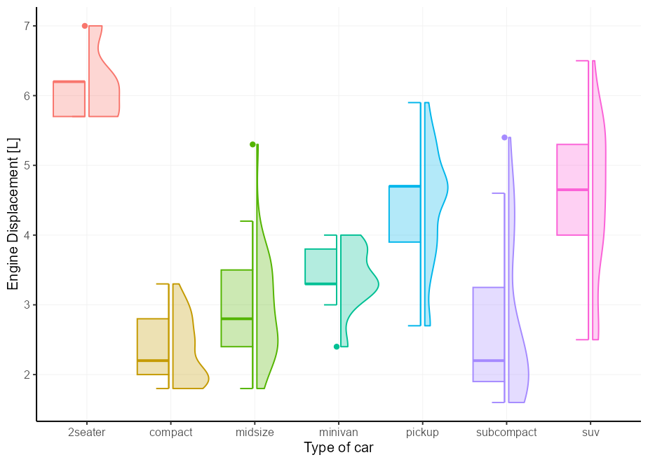
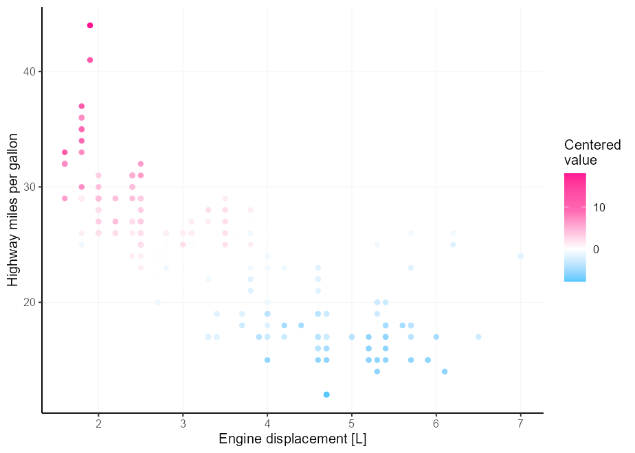
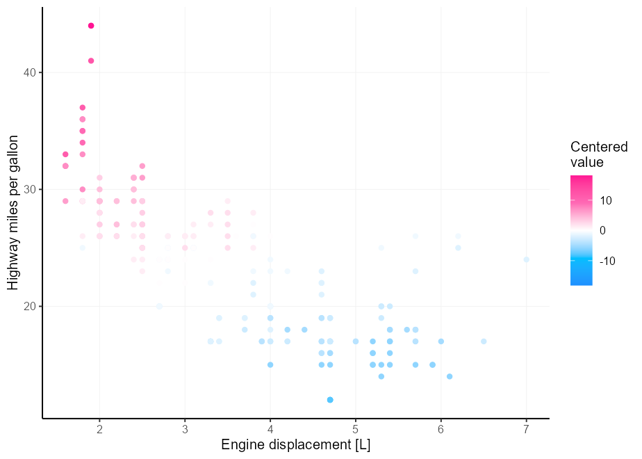
假設您的顏色直覺比我擁有的更好,而三種顏色不足以滿足您的不同調色板需求。一個痛苦的地方是,如果您的極限並不完美地圍繞它,那麼獲得中點很棘手。使用scales::rescale_mid()輸入聯盟中的rescaler論點。
 my_palette <- c( " dodgerblue " , " deepskyblue " , " white " , " hotpink " , " deeppink " )

p <- ggplot( mpg , aes( displ , hwy , colour = cty - mean( cty ))) +
  geom_point() +
  labs(
    x = " Engine displacement [L] " ,
    y = " Highway miles per gallon " ,
    colour = " Centered n value "
  )

p +
  scale_colour_gradientn(
    colours = my_palette ,
    rescaler = ~ rescale_mid( .x , mid = 0 )
  )
另一種選擇是簡單地將限制置於x上。我們可以通過為量表的限制提供功能來做到這一點。
 p +
  scale_colour_gradientn(
    colours = my_palette ,
    limits = ~ c( - 1 , 1 ) * max(abs( .x ))
  )
您可以用geom_text()標記點,但是潛在的問題是文本和指向重疊。
set.seed( 0 )
df <- USArrests [sample(nrow( USArrests ), 5 ), ]
df $ state <- rownames( df )

q <- ggplot( df , aes( Murder , Rape , label = state )) +
  geom_point()
q + geom_text()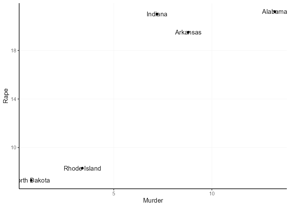
這個問題有幾種典型的解決方案,它們都有缺點:
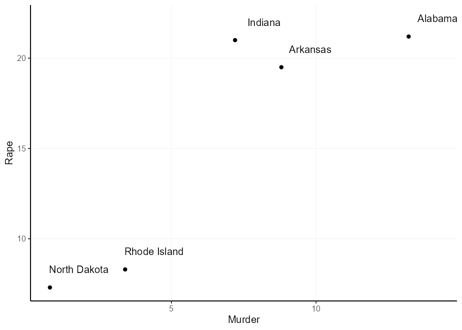
nudge_x和nudge_y參數。這裡的問題是這些是在數據單元中定義的,因此間距是不可預測的,並且無法將其取決於原始位置。hjust和vjust美學。它使您可以依靠原始位置,但是它們沒有天然偏移。這是行動中的選項2和3:
 q + geom_text( nudge_x = 1 , nudge_y = 1 )

q + geom_text(aes(
  hjust = Murder > mean( Murder ),
  vjust = Rape > mean( Rape )
))
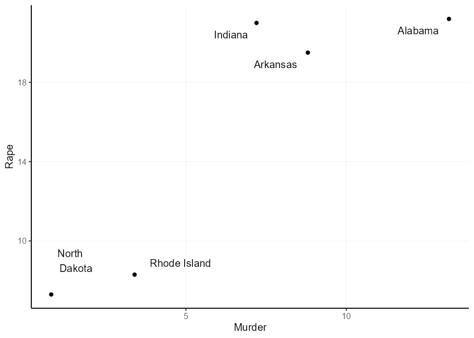
您可能會想:“我可以將理由倍增以獲得更廣泛的偏移”,而您是對的。但是,由於理由取決於文本的大小,因此您可能會獲得不平等的偏移。請注意,在下面的情節中,“北達科他州”在Y方向上的偏見和X方向的“羅德島”過於偏見。
 q + geom_text(aes(
  label = gsub( " North Dakota " , " North n Dakota " , state ),
  hjust = (( Murder > mean( Murder )) - 0.5 ) * 1.5 + 0.5 ,
  vjust = (( Rape > mean( Rape )) - 0.5 ) * 3 + 0.5
))
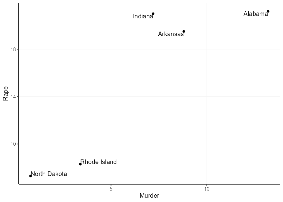
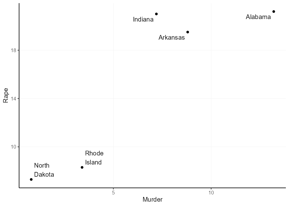
geom_label()的好處是您可以關閉標籤框並保留文本。這樣,您可以繼續使用其他有用的東西,例如label.padding設置,以使文本從文本到標籤的絕對(數據無關)偏移。
 q + geom_label(
  aes(
    label = gsub( " " , " n " , state ),
    hjust = Murder > mean( Murder ),
    vjust = Rape > mean( Rape )
  ),
  label.padding = unit( 5 , " pt " ),
  label.size = NA , fill = NA
)
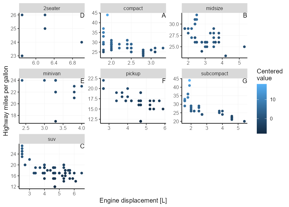
這曾經是將刻面標籤放入面板中的提示,曾經很複雜。使用GGPLOT2 3.5.0,您不再需要擺弄設置無限位置並調整hjust或vjust參數。現在,您可以使用x = I(0.95), y = I(0.95)將文本放在右上角。打開細節以查看舊提示。
將文本註釋放在刻面圖上是一個痛苦,因為限制可能會在每面板上有所不同,因此很難找到正確的位置。探索減輕這種痛苦的擴展是標記延伸,但我們可以在Vanilla GGPLOT2中做類似的事情。
幸運的是,GGPLOT2的位置軸中有一個機械師,讓我們的-Inf和Inf分別解釋為量表的最小和最大極限3 。您可以通過選擇x = Inf, y = Inf將標籤放在角落中來利用這一點。您也可以使用-Inf而不是Inf放置在底部而不是頂部,也可以將其放在左上而不是右。
我們需要將hjust / vjust參數與情節側面匹配。對於x/y = Inf ,它們需要為hjust/vjust = 1 ,對於x/y = -Inf它們需要為hjust/vjust = 0 。
 p + facet_wrap( ~ class , scales = " free " ) +
  geom_text(
    # We only need 1 row per facet, so we deduplicate the facetting variable
    data = ~ subset( .x , ! duplicated( class )),
    aes( x = Inf , y = Inf , label = LETTERS [seq_along( class )]),
    hjust = 1 , vjust = 1 ,
    colour = " black "
  )
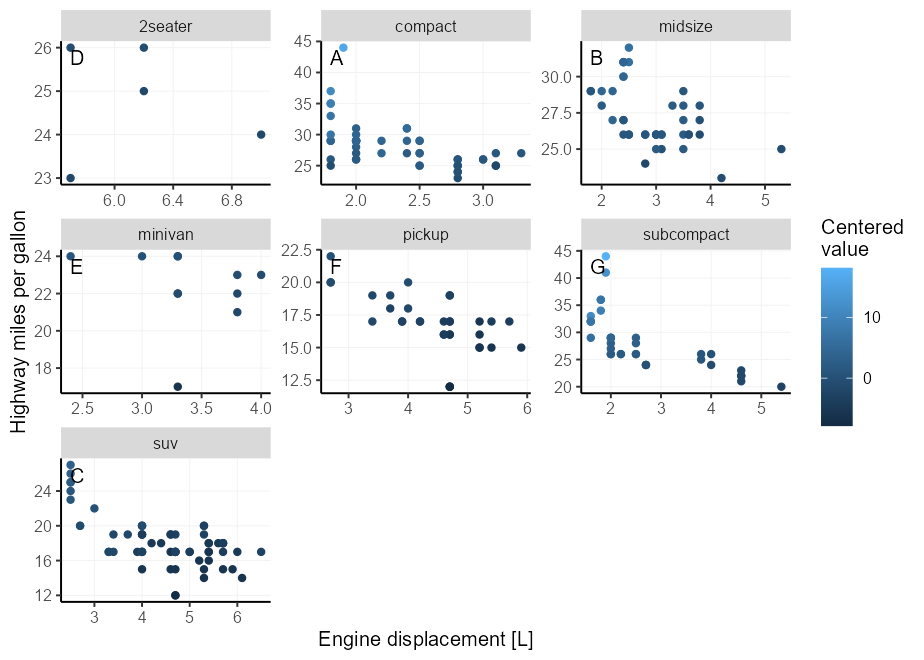
不幸的是,這將文字直接放在面板的邊界,這可能會冒犯我們的美麗感。通過使用geom_label() ,我們可以變得更加典型,這使我們可以通過設置label.padding參數來精確地控製文本和麵板邊界之間的間距。
此外,我們可以使用label.size = NA, fill = NA隱藏GEOM的文本框部分。出於插圖目的,我們現在將標籤放在左上角而不是右上角。
 p + facet_wrap( ~ class , scales = " free " ) +
  geom_label(
    data = ~ subset( .x , ! duplicated( class )),
    aes( x = - Inf , y = Inf , label = LETTERS [seq_along( class )]),
    hjust = 0 , vjust = 1 , label.size = NA , fill = NA ,
    label.padding = unit( 5 , " pt " ),
    colour = " black "
  )
假設我們的任務是製作一堆類似的圖,並具有不同的數據集和列。例如,我們可能想用一些特定的預設製作一系列的小花4 :我們希望條能觸摸X軸而不是繪製垂直網格線。
製作一堆類似地塊的一種眾所周知的方法是將情節構造包裹在一個功能中。這樣,您可以在功能中使用所需的所有預設。
我的情況您可能不知道,使用aes()函數進行編程的各種方法,而使用{{ }} (curly-curly)是更靈活的方法5 。
 barplot_fun <- function ( data , x ) {
  ggplot( data , aes( x = {{ x }})) +
    geom_bar( width = 0.618 ) +
    scale_y_continuous( expand = c( 0 , 0 , 0.05 , 0 )) +
    theme( panel.grid.major.x = element_blank())
}

barplot_fun( mpg , class )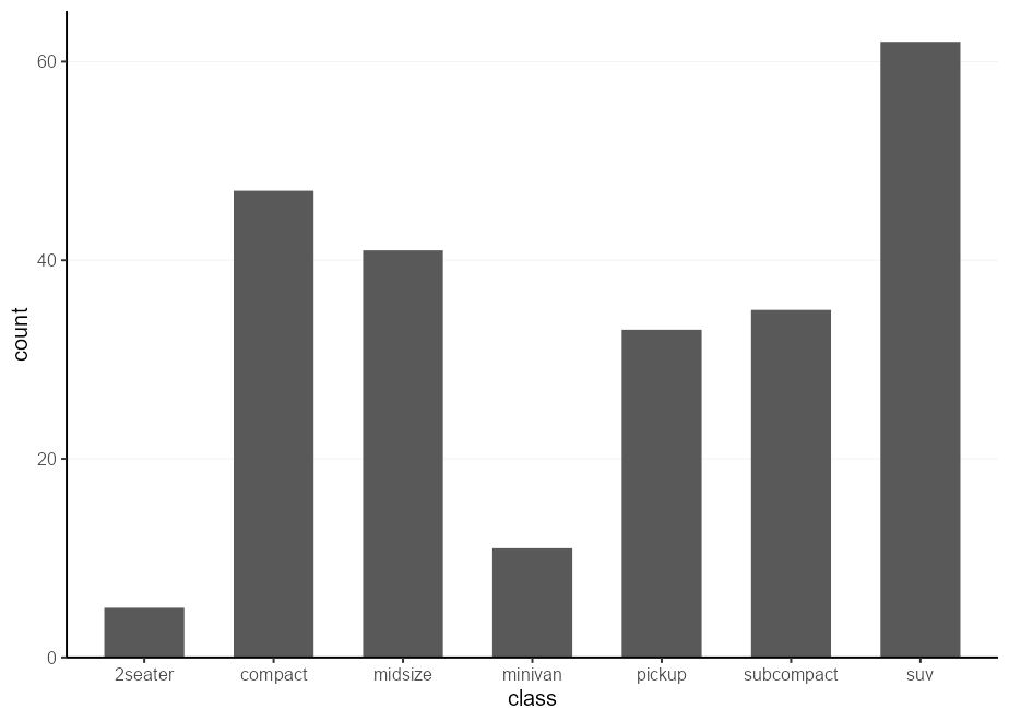
這種方法的一個缺點是,您可以在函數參數中鎖定任何美學。為了解決這個問題,更簡單的方法就是簡單地將...直接傳遞到aes() 。
 barplot_fun <- function ( data , ... ) {
  ggplot( data , aes( ... )) +
    geom_bar( width = 0.618 ) +
    scale_y_continuous( expand = c( 0 , 0 , 0.1 , 0 )) +
    theme( panel.grid.major.x = element_blank())
}

barplot_fun( mpg , class , colour = factor ( cyl ), !!! my_fill )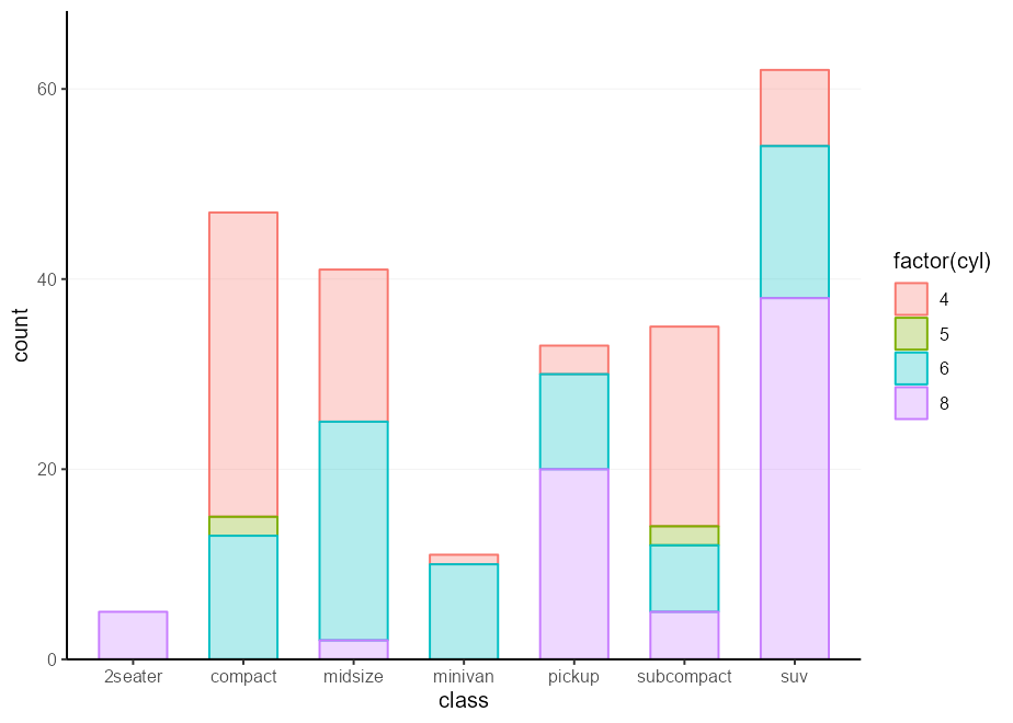
做非常相似的方法是使用“骨架”。骨骼背後的想法是,您可以在有或沒有任何data參數的情況下構建繪圖,並以後添加細節。然後,當您實際想製作繪圖時,可以使用%+%填充或替換數據集,以及+ aes(...)來設置相關的美學。
 barplot_skelly <- ggplot() +
  geom_bar( width = 0.618 ) +
  scale_y_continuous( expand = c( 0 , 0 , 0.1 , 0 )) +
  theme( panel.grid.major.x = element_blank())

my_plot <- barplot_skelly % + % mpg +
  aes( class , colour = factor ( cyl ), !!! my_fill )
my_plot 
關於這些骨架的一件事是,即使您已經填寫了data和mapping參數,也可以一次又一次地替換它們。
 my_plot % + % mtcars +
  aes( factor ( carb ), colour = factor ( cyl ), !!! my_fill )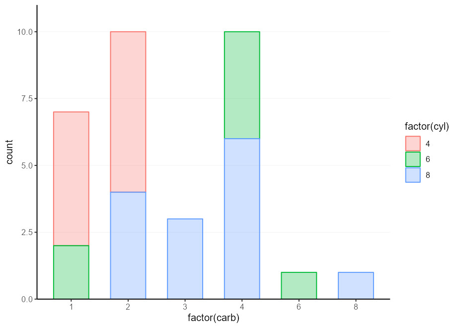
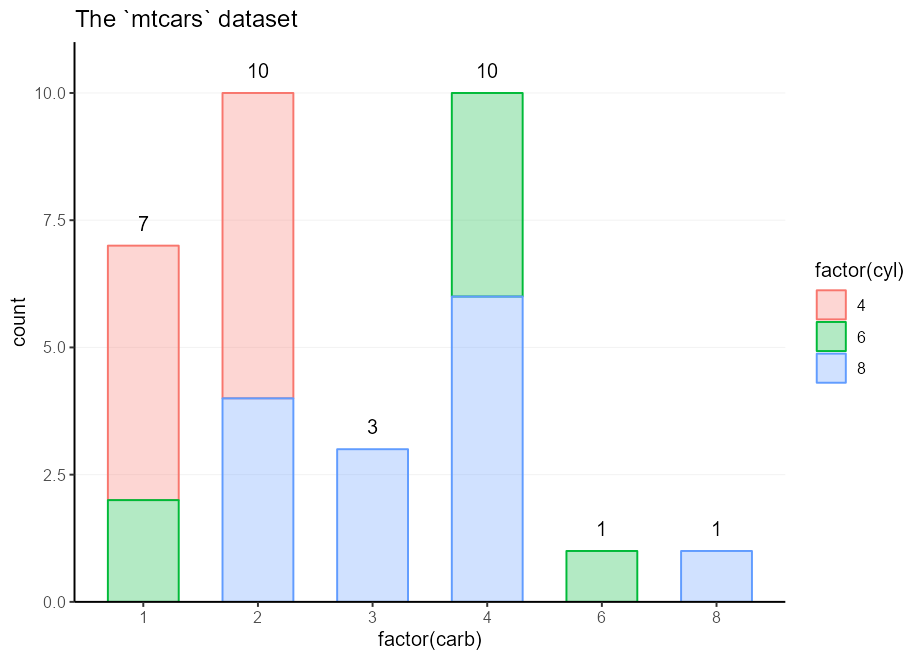
這裡的想法是不是要骨骼整個圖,而只是一組經常使用的零件。例如,我們可能想標記您的小號,並將所有構成標記為Barplot的東西打包在一起。訣竅是不要將這些組件與+一起添加在一起,而只是將它們放入list() 。然後,您可以+您的列表以及主繪圖調用。
 labelled_bars <- list (
  geom_bar( my_fill , width = 0.618 ),
  geom_text(
    stat = " count " ,
    aes( y     = after_stat( count ),
        label = after_stat( count ),
        fill  = NULL , colour = NULL ),
    vjust = - 1 , show.legend = FALSE
  ),
  scale_y_continuous( expand = c( 0 , 0 , 0.1 , 0 )),
  theme( panel.grid.major.x = element_blank())
)

ggplot( mpg , aes( class , colour = factor ( cyl ))) +
  labelled_bars +
  ggtitle( " The `mpg` dataset " )

ggplot( mtcars , aes( factor ( carb ), colour = factor ( cyl ))) +
  labelled_bars +
  ggtitle( " The `mtcars` dataset " )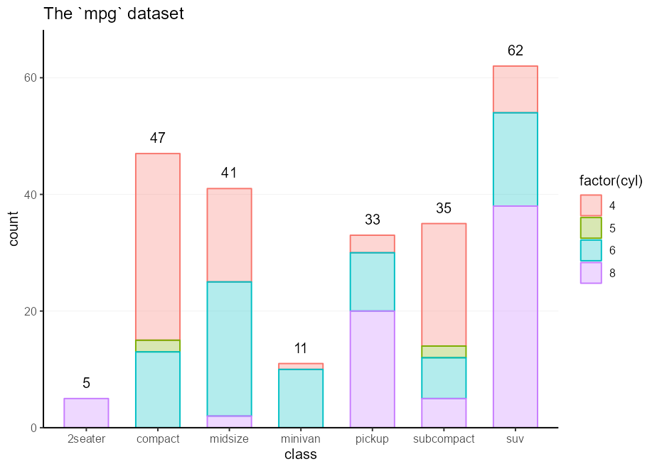
 #> ─ Session info ───────────────────────────────────────────────────────────────
#>  setting  value
#>  version  R version 4.3.2 (2023-10-31 ucrt)
#>  os       Windows 11 x64 (build 22631)
#>  system   x86_64, mingw32
#>  ui       RTerm
#>  language (EN)
#>  collate  English_Netherlands.utf8
#>  ctype    English_Netherlands.utf8
#>  tz       Europe/Amsterdam
#>  date     2024-02-27
#>  pandoc   3.1.1
#>
#> ─ Packages ───────────────────────────────────────────────────────────────────
#>  package     * version    date (UTC) lib source
#>  cli           3.6.2      2023-12-11 []  CRAN (R 4.3.2)
#>  colorspace    2.1-0      2023-01-23 []  CRAN (R 4.3.2)
#>  digest        0.6.34     2024-01-11 []  CRAN (R 4.3.2)
#>  dplyr         1.1.4      2023-11-17 []  CRAN (R 4.3.2)
#>  evaluate      0.23       2023-11-01 []  CRAN (R 4.3.2)
#>  fansi         1.0.6      2023-12-08 []  CRAN (R 4.3.2)
#>  farver        2.1.1      2022-07-06 []  CRAN (R 4.3.2)
#>  fastmap       1.1.1      2023-02-24 []  CRAN (R 4.3.2)
#>  generics      0.1.3      2022-07-05 []  CRAN (R 4.3.2)
#>  ggplot2     * 3.5.0.9000 2024-02-27 []  local
#>  glue          1.7.0      2024-01-09 []  CRAN (R 4.3.2)
#>  gtable        0.3.4      2023-08-21 []  CRAN (R 4.3.2)
#>  highr         0.10       2022-12-22 []  CRAN (R 4.3.2)
#>  htmltools     0.5.7      2023-11-03 []  CRAN (R 4.3.2)
#>  knitr         1.45       2023-10-30 []  CRAN (R 4.3.2)
#>  labeling      0.4.3      2023-08-29 []  CRAN (R 4.3.1)
#>  lifecycle     1.0.4      2023-11-07 []  CRAN (R 4.3.2)
#>  magrittr      2.0.3      2022-03-30 []  CRAN (R 4.3.2)
#>  munsell       0.5.0      2018-06-12 []  CRAN (R 4.3.2)
#>  pillar        1.9.0      2023-03-22 []  CRAN (R 4.3.2)
#>  pkgconfig     2.0.3      2019-09-22 []  CRAN (R 4.3.2)
#>  R6            2.5.1      2021-08-19 []  CRAN (R 4.3.2)
#>  ragg          1.2.7      2023-12-11 []  CRAN (R 4.3.2)
#>  rlang         1.1.3      2024-01-10 []  CRAN (R 4.3.2)
#>  rmarkdown     2.25       2023-09-18 []  CRAN (R 4.3.2)
#>  rstudioapi    0.15.0     2023-07-07 []  CRAN (R 4.3.2)
#>  scales      * 1.3.0      2023-11-28 []  CRAN (R 4.3.2)
#>  sessioninfo   1.2.2      2021-12-06 []  CRAN (R 4.3.2)
#>  systemfonts   1.0.5      2023-10-09 []  CRAN (R 4.3.2)
#>  textshaping   0.3.7      2023-10-09 []  CRAN (R 4.3.2)
#>  tibble        3.2.1      2023-03-20 []  CRAN (R 4.3.2)
#>  tidyselect    1.2.0      2022-10-10 []  CRAN (R 4.3.2)
#>  utf8          1.2.4      2023-10-22 []  CRAN (R 4.3.2)
#>  vctrs         0.6.5      2023-12-01 []  CRAN (R 4.3.2)
#>  viridisLite   0.4.2      2023-05-02 []  CRAN (R 4.3.2)
#>  withr         3.0.0      2024-01-16 []  CRAN (R 4.3.2)
#>  xfun          0.41       2023-11-01 []  CRAN (R 4.3.2)
#>  yaml          2.3.8      2023-12-11 []  CRAN (R 4.3.2)
#>
#>
#> ──────────────────────────────────────────────────────────────────────────────
好吧,您需要在文檔開始時進行一次。但是再也不會!除了您的下一個文檔。只需在您的文檔中編寫一個plot_defaults.R腳本和source()即可。每個項目的複制腳本。然後,確實,再也不會再:心:。 ↩
這是一個謊言。實際上,我使用aes(colour = after_scale(colorspace::darken(fill, 0.3)))而不是減輕填充。不過,我不希望此讀數對{Colorspace}具有依賴性。 ↩
除非您通過設置oob = scales::oob_censor_any來自我破壞圖,否則在刻度中。 ↩
在您的靈魂中,您真的想製作一堆小花嗎? ↩
另一種選擇是使用.data代詞,如果要提前鎖定該列,則可以是.data[[var]] .data$var ,或者當var作為字符傳遞時。 ↩
這個位最初稱為“部分骨架”,但由於胸腔是骨骼的一部分,因此這個標題聽起來更令人回味。 ↩


